Do tabular foundation models repair themselves?
Abstract. Ablation is the workhorse of mechanistic interpretability: we delete a component, measure the damage, and read the damage as the component’s importance. Self-repair breaks this inference: downstream components compensate for the deleted one and the output recovers, so the damage understates what the component does. Self-repair has been quantified in language models [1]. A recent study of tabular foundation models (TFMs) [5] reports that they self-repair as well. However, the criterion that study adopts does not separate self-repair from mere redundancy. In this paper we measure the quantity that does, i.e., the direct effect of a layer, using a causal intervention known as path patching. We evaluate four state-of-the-art TFMs on 15 binary classification tasks and find that the recovery is passive redundancy rather than active repair.
A 5-minute video overview of this work is also available.
Table of contents
- 1. Introduction
- 2. Self-repair: definition and how prior work quantifies it
- 3. Self-repair in TFMs: the prior claim and what it identifies
- 4. Measuring the direct effect in TFMs
- 5. Experiments
- 6. Conclusion
- 7. Reproducibility
- References
- Appendix A: the layer-skipping experiment on all four models
- Appendix B: ablation diagnostics on all four models
- Appendix C: two further checks on the compensation effect
1. Introduction
Mechanistic interpretability rests on a simple inference. We ablate a component (e.g., a layer or an attention head), observe how much the output degrades, and attribute the degradation to the component’s function. The inference is only valid if the rest of the network does not react to the ablation. Self-repair is the phenomenon that breaks this assumption: after a component is removed, downstream components change what they compute and restore part of the lost output. The consequence is that ablation-based importance systematically underestimates the components that matter most. This has been documented repeatedly in language models [1, 2, 3, 4].
Tabular foundation models are transformers that solve a supervised tabular task by in-context learning. A single forward pass consumes the entire data table, i.e., the labelled support rows together with the unlabelled query rows, and emits predictions for the query rows, with no gradient step and no task-specific fitting. What matters below is that the input table stays in context for the whole forward pass, so any layer can recompute from it.
Self-repair has been quantified only in language models. Balef et al. [5] give the first mechanistic study of layerwise dynamics in TFMs and report that self-repair occurs in the middle and late layers of most of them. However, their criterion is the shape of a trajectory: after skipping a layer they decode at every subsequent depth and read a drop followed by a recovery of ROC AUC as evidence of repair. That reading presupposes a mechanism we call active repair, in which the downstream layers respond to the missing write. A second mechanism, passive redundancy, produces the same trajectory: if the information written by the skipped layer is duplicated elsewhere, the downstream layers recover the output without changing what they write.
We study whether TFMs exhibit self-repair in the causal sense in which it is defined for language models, i.e., as a change in what the downstream layers compute. Balef et al. define it by its outcome, i.e., the decoded performance recovers after an ablation. They pose the right dichotomy (redundancy or repair), but that definition is satisfied by both alternatives. We resolve the dichotomy with a quantity their design does not contain: the direct effect [1], measured via path patching [2].
In summary, we make the following contributions:
- We show that the criterion of [5] cannot establish self-repair, because it does not separate repair from redundancy.
- To separate self-repair from redundancy, we propose an additional measurement of the direct effect of layers, obtained by path patching [2].
- Based on the proposed measurement and on results for 4 SOTA TFMs and 15 tasks, we draw a different conclusion from that of [5]: the performance recovery reported for TFMs is passive redundancy.
- In addition, we make two further measurement choices, using logit margin in place of ROC AUC and resample ablation in place of zero ablation. Both make the experimental results easier to read.
Why this matters for safety. TFMs are deployed on high-stakes tabular decisions, e.g., lending and clinical prediction, so models need to be trustworthy. Mechanistic interpretability bridges the gap by identifying the components responsible for a behaviour, and ablation is the cheapest and most widely used technique. Self-repair is the failure mode that invalidates it. As noted above, an audit built on ablation may return false assurance. Our contribution to AI safety is twofold: (i) we point out the criterion previously used to claim self-repair in TFMs cannot establish it, so the direct effect is required instead; and (ii) we measure the direct effect and find no compensation, i.e., for these models ablation-based attribution is not corrupted in this way. We stress that the second statement is based on a limited set of models and tasks, and does not carry over to the general case.
2. Self-repair: definition and how prior work quantifies it
Intuition. The intuition behind self-repair is that a network reacts to its own damage. When a component is removed, the components downstream of it see a different residual stream, and they may respond by writing something different from what they would have written otherwise. Self-repair is the case in which that response pushes the output back towards its undamaged value. Note that the definition is a statement about the downstream reaction, not about the output: an output that barely moves is compatible with a strong reaction (e.g., active repair) and with no reaction at all (e.g., passive redundancy).
Causal model. The network can be viewed as a causal model [6] in which \(A\) denotes the component under study (e.g., a layer or an attention head), \(B\) denotes everything downstream of \(A\), and \(y\) denotes a scalar output of the final decoder that measures how strongly the model favours the correct class. We restrict attention to binary classification throughout.
Three effects. Figure 1 defines the three effects used throughout this paper.
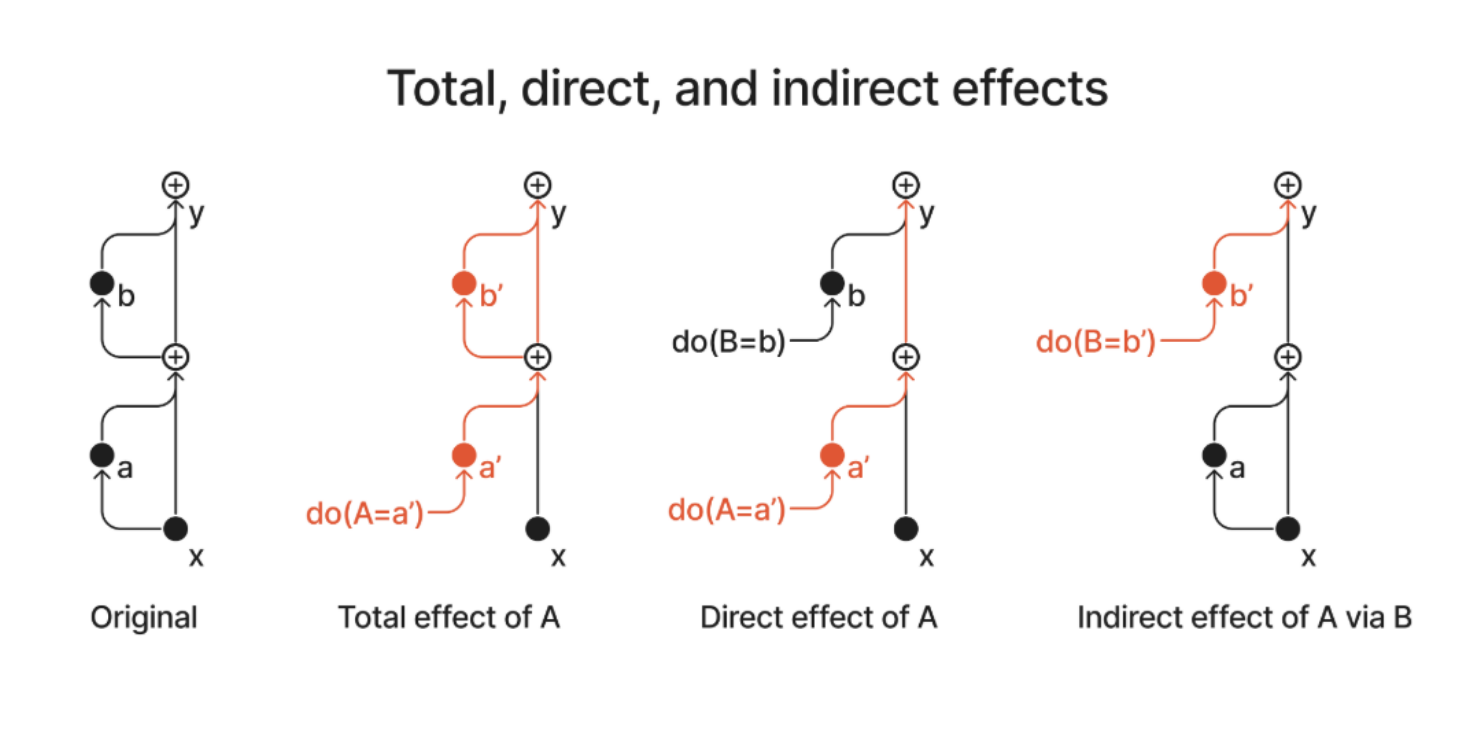 Figure 1: Original is the clean pass, in which \(a\) and \(b\) take their clean values. The three effects differ only in which nodes the intervention reaches: \(do(A = a’)\) substitutes \(A\)’s output, and \(do(B = b)\) fixes \(B\) to its clean value so that the intervention does not impact it. Illustration taken from [1].
The “Original” panel shows the clean pass (without any intervention), and the value a component takes in it is referred to as its clean value. Let \(\tilde{a}\) be the value we substitute for \(A\)’s output, written \(a’\) in the figure. The three effects differ only in what we allow to react.
- The total effect \(TE\) is the change in \(y\) when we set \(A = \tilde{a}\) and let \(B\) react freely.
- The direct effect \(DE\) is the change in \(y\) when we set \(A = \tilde{a}\) and simultaneously freeze \(B\) at its clean values, so that only the path \(A \to y\) carries the intervention.
- The indirect effect \(IE\) is the change in \(y\) when we leave \(A\) clean and set \(B\) to the values it would take under the intervention, so that only the path \(A \to B \to y\) carries it.
The three are related by \(TE = DE + IE\). Following [1] we define the compensation effect
\[CE = DE - TE = -IE ,\]and we say that a component self-repairs if \(CE > 0\), i.e., if the damage that reaches the output is smaller than the component’s own direct contribution. Note that \(CE < 0\) means the downstream reaction amplifies the loss and \(CE = 0\) means the downstream layers are passive.
Why both \(TE\) and \(DE\) are needed. It is easy to see that neither effect alone identifies self-repair. Consider a toy network with two components, \(A\) and \(B\), writing values \(a\) and \(b\) into a shared stream. Component \(A\) constantly writes \(a = 1\), and the output is read as
\[y = \begin{cases} 1 & \text{if } a + b > 0 \\ 0 & \text{otherwise.}\end{cases}\]The intervention is \(do(A = 0)\). We consider three scenarios, which differ only in the rule \(B\) follows.
| scenario | \(B\)’s rule | \(a + b\) | \(y\) | \(TE\) | \(DE\) |
|---|---|---|---|---|---|
| ① redundant | \(b = 1\) always | \(2\) | \(1\) | \(0\) | \(0\) |
| ② repaired | \(b = 1 - a\) | \(1\) | \(1\) | \(0\) | \(1\) |
| ③ load-bearing | \(b = 0\) always | \(1\) | \(1\) | \(1\) | \(1\) |
Table 1: three scenarios that are indistinguishable at the clean output, all producing \(y = 1\). The last two columns are the effects of \(do(A = 0)\).
The total effect is \(0\) in both ① and ②, and therefore cannot separate them. The direct effect is \(1\) in both ② and ③, and therefore cannot separate them either. Only the gap singles out ②, since \(CE\) is non-zero there and zero in ① and ③.
Quantification in language models. The authors of [1] evaluate a 7B-parameter Chinchilla model on 1209 factual-recall prompts, ablating one attention layer at a time. They obtain \(DE\) by unembedding the layer’s own output directly, and \(TE\) by ablating the layer and reading the final logits. Figure 2 shows their key result: the point cloud of \((DE, TE)\) pairs sits predominantly below the diagonal \(y = x\), i.e., \(TE < DE\) for a large fraction of (layer, prompt) pairs. Ablation on its own yields only \(TE\), so it cannot produce this picture at all. The direct effect has to be measured separately, and the mass below the diagonal is the empirical signature of \(CE > 0\).
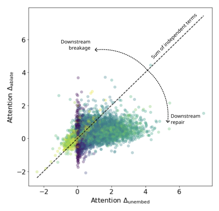 Figure 2: direct effect against total effect in a language model. One point is one (layer, prompt) pair, coloured by layer depth. Mass below the diagonal is the signature of self-repair. Taken from Figure 2c of [1].
Moreover, the compensation is proportional. Regressing \(CE\) on \(DE\) across prompts, layer by layer, they find a tight linear relation in the middle and late layers, peaking at layer 23 with \(R^2 = 0.92\) and slope \(0.69\) (Figures 4b and 4d of [1]).1 We adopt both as our reference, since a scattered relation would indicate coincidence rather than a mechanism.
3. Self-repair in TFMs: the prior claim and what it identifies
We proceed in three steps: (i) what Balef et al. do and what they conclude; (ii) the main argument that their criterion cannot identify self-repair; and (iii) two of their measurement choices that make the phenomenon harder to see.
3.1 What Balef et al. do
Balef et al. [5] study six state-of-the-art TFMs. Their self-repair experiment has four parts.
- Instrument: the tabular logit lens. A TFM’s native decoder expects the representation of the final layer, so they train a separate decoder for every layer and use it to measure the performance of that layer.
- Intervention: layer skipping. They remove one layer and apply the lens at every subsequent layer, which gives a trajectory of performance scores.
- Criterion: they state that, if the TFM can recover from dropping a layer, it has learned to self-repair, and layers overlap in functionality.
- Conclusion: self-repair generally occurs after layer ablations, except for the early layers.
Figure 3 shows our reproduction of this experiment. Skipping an early layer produces a drop that persists to the output, whereas skipping a middle or late layer produces a drop that closes well before the final layer.
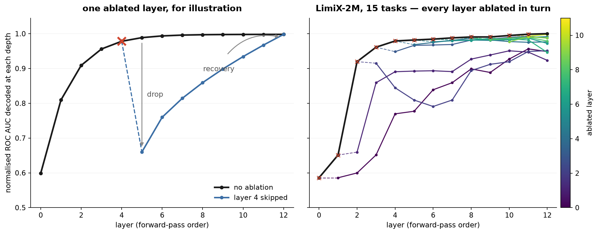 Figure 3: the layer-skipping experiment in [5]. Left (for illustration): ablating one layer. The black baseline is the unablated trajectory, the red cross marks the skipped layer, and the decoded performance drops at the next depth and then recovers. Right: the same experiment on LimiX-2M over 15 tasks, with every layer ablated in turn; one coloured curve is one skipped layer, i.e., one instance of the left panel. Early layers do not recover, middle and late layers do. The other three models are in Appendix A. All four agree with what the paper reports, including the two models [5] does not study.
The authors pose the dichotomy themselves. They admit, in their own words, that it is unclear whether the robustness to layer ablation comes from self-repair or from layer redundancy, since performance has been measured only at the final layer. Their diagnosis is that too few depths are measured and they remedy it by measuring all of them. In contrast, we argue below that the number of depths is not what the dichotomy turns on.
3.2 The criterion cannot identify self-repair
Their criterion defines self-repair by its outcome, i.e., by the shape of the trajectory, whereas we argue it should rest on the mechanism. The distinction matters because an outcome criterion only ever sees \(TE\), and \(TE\) is near zero under both mechanisms. Telling them apart requires the gap \(CE = DE - TE\).
We now state the main argument, which is independent of how performance is measured. The two mechanisms differ in what the downstream layers write, so we track that quantity directly. Let the network have \(L\) layers and let \(m\) be the layer that is skipped. For any layer \(\ell\), write \(a_\ell\) for the value it writes into the residual stream in the clean pass and \(\hat{a}_\ell\) for what it writes in the ablated pass.
- Under active repair, the downstream layers respond to the missing write, so \(\hat{a}_\ell \neq a_\ell\) for \(\ell > m\), and the recovery is produced by that response.
- Under passive redundancy, the downstream layers write exactly what they always write, \(\hat{a}_\ell = a_\ell\), and the recovery occurs because the information carried by \(a_m\) is duplicated in the residual stream and in the input table, which remains in context.
Both produce a drop at depth \(m+1\), where \(a_m\) is simply absent from the residual stream, and both produce a recovery by depth \(L\). The two mechanisms draw the same curve, and every curve in Figure 3 admits both explanations. Therefore the trajectory criterion cannot decide between them.
3.3 Two measurement choices
Two further choices in the design of [5] make self-repair harder to see. Note that they are independent of the argument above.
- Performance is measured by ROC AUC (e.g., see Figure 3), which is rank-based and saturates: once an early layer separates the classes, later layers can sharpen or suppress the true class without moving the metric, so a flat ROC AUC curve is uninformative about what the late layers do.
- Layers are removed by skipping, which is a form of zero ablation. Zero ablation sets a component’s contribution to a value the network may never encounter during training. In other words, the resulting perturbation is not representative.
We propose alternatives in Section 4.
4. Measuring the direct effect in TFMs
In Sections 4.1 and 4.2, we explain how to measure \(TE\) and \(DE\), and state the criterion that resolves the dichotomy. In Sections 4.3 and 4.4, we improve the two measurement choices of Section 3.3 to make the resulting quantities more readable.
4.1 The direct effect via path patching
We follow the path-patching construction of [2]. The main idea is to change what layer \(m\) writes and let no other layer notice. Formally, let \(r_\ell\) denote the residual stream after layer \(\ell\) and \(a_m = r_m - r_{m-1}\) the write of layer \(m\). We refer to a value substituted for \(a_m\) as a source write, denoted \(\tilde{a}_m\) (Section 4.4 says where it comes from). We substitute it and keep every downstream write \(a_\ell\), \(\forall \ell > m\), at its clean value. That is, nothing is recomputed on the perturbed residual stream. This gives
\[r_L^{DE}(m) = r_L^{\text{clean}} - a_m + \tilde{a}_m .\]The total effect is obtained from the same substitution with the downstream layers free to react, i.e., by re-running the forward pass, and read through the same native decoder. Figure 4 contrasts the two.
The two effects in code
# inputs:
# - table: the data table
# - m: the ablated layer

clean   = forward(table)
a       = clean.writes             # a[0..L-1]; a[l] is what layer l writes into the residual stream
r_clean = clean.residual           # the final residual
a_tilde = source_write(m)          # the substitute for a[m]; Section 4.4 says where it comes from

# total effect: rerun the forward pass, downstream reacts
r_te = forward(table, patch={m: a_tilde}).residual
te   = decode(r_te) - decode(r_clean)

# direct effect: no rerun, every downstream write reused
r_de = r_clean - a[m] + a_tilde
de   = decode(r_de) - decode(r_clean)

ce = de - te
Three things are visible here.
- Only the total-effect branch calls
forwardagain, so the direct effect is arithmetic on the recorded residual. - Both branches call the same
decode, which is the model’s native decoder. - The two branches differ in one place only, namely whether the downstream writes are recomputed.
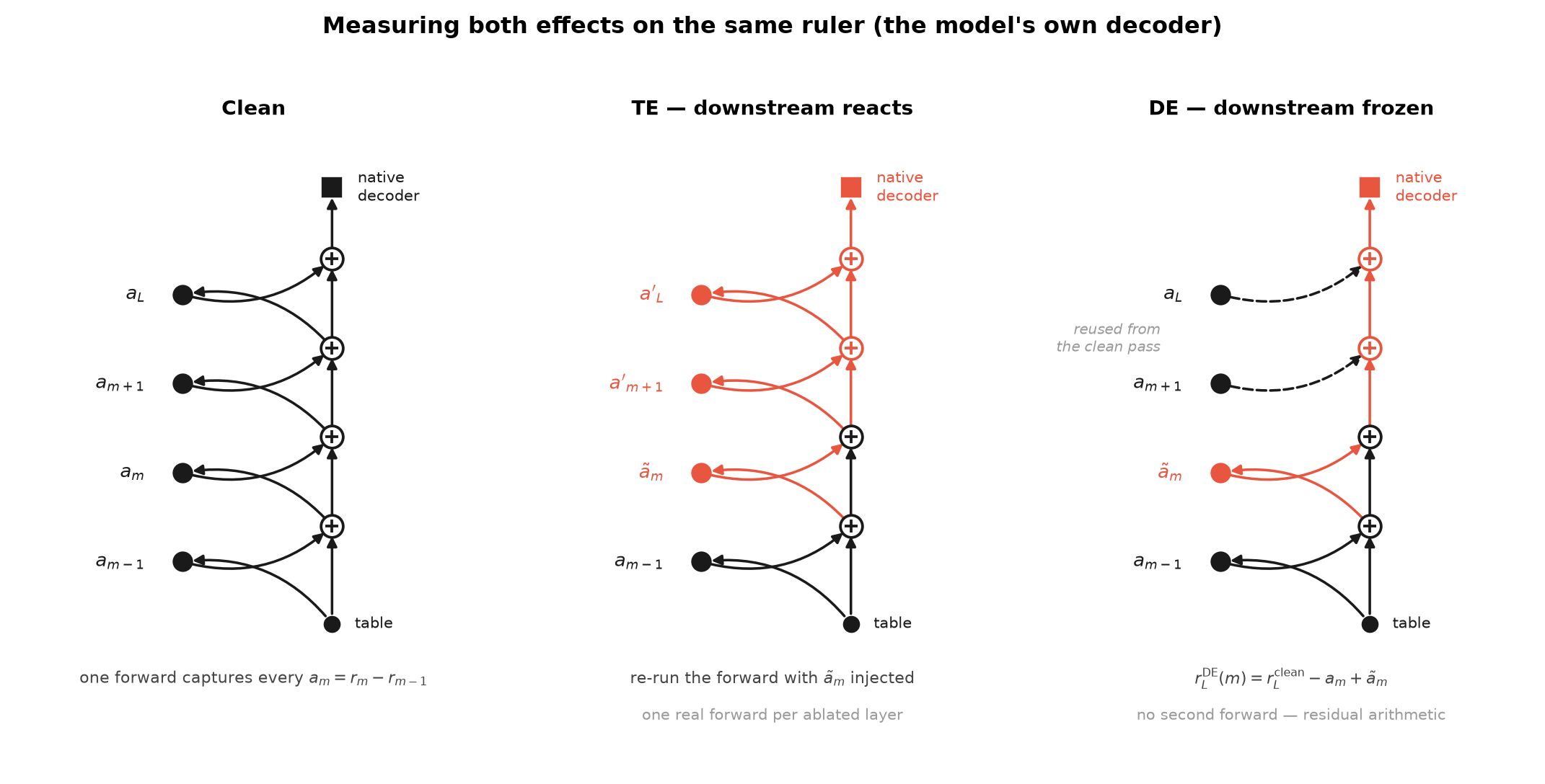 Figure 4: the clean pass, the total effect, and the direct effect. The direct effect requires no second forward pass, since reusing the recorded downstream writes reduces to arithmetic on the clean residual.
Both effects are read on the same scale (the model’s own decoder), which is what makes their difference meaningful. This rules out the per-depth decoders of the tabular logit lens [5], which give each depth its own scale, and it differs from [1], who read \(DE\) by unembedding \(a_m\) alone rather than decoding the patched residual.
4.2 Criterion
Given \(DE\) and \(TE\) we compute \(CE = DE - TE\) and apply the criterion of Section 2. We say that a model exhibits self-repair if
- the \((DE, TE)\) cloud has mass below the diagonal with \(CE > 0\) of a magnitude comparable to \(DE\), and
- \(CE\) grows with \(DE\) in a tight per-layer regression, as in language models.
We require both. The first is qualitative, i.e., compensation is present at all; the second is quantitative, i.e., it is systematic rather than incidental.
4.3 Logit margin instead of ROC AUC
To address the saturation issue of ROC AUC discussed in Section 3.3, we propose to measure performance by the logit margin.
For a binary task on query row \(i\), with true-class logit \(z_{i,y_i}\) and competitor logit \(z_{i,1-y_i}\), we compute it in three steps.
- Per-row margin: \(\gamma_i = z_{i,y_i} - z_{i,1-y_i}\).
- Normalize: \(\hat\gamma_i = \gamma_i / \lvert \bar\gamma^{\text{clean}} \rvert\), where \(\bar\gamma^{\text{clean}}\) is the clean final-layer margin of the same task. The sign is unchanged, so \(0\) remains the model’s decision boundary and a negative value still indicates a flipped decision. Normalization adds a unit: every margin we report below is a multiple of \(\bar\gamma^{\text{clean}}\), so \(1\) is the clean final confidence and values \(> 1\) indicate overconfidence.
- [Optional] median over rows: \(\operatorname{median}_i \hat\gamma_i\). We use the median rather than the mean because the median is more robust to heavy-tailed distributions. We aggregate throughout because it makes the figures easier to read; Appendix C reports the per-row version.
Section 5.2 empirically validates our proposal.
4.4 Resample ablation instead of zero ablation
To address the out-of-distribution issue of zero ablation discussed in Section 3.3, we propose to use resample ablation [7]. The intuition is to replace what a layer says instead of deleting it, so that the residual stream stays in the range the model was trained on.
We refer to the table whose effects we are measuring as the target table, and to a table we take the source write \(\tilde{a}_m\) from as a source table. The intervention then asks what the layer would have contributed on other data, rather than what happens when it produces nothing at all.
Formally, let \(T\) be the target table and \(T^{(1)}, \dots, T^{(K)}\) be \(K\) source tables drawn from the same task, and write \(a_m(T)\) for the write layer \(m\) produces on \(T\). A source table has a different number of rows and features, so we fill each position \(p\) of the source write by drawing uniformly from the source positions of the same role, i.e., support rows from support rows and query rows from query rows:2
\[\tilde{a}^{(k)}_m[p] = a_m\big(T^{(k)}\big)\big[\pi_k(p)\big], \qquad \pi_k(p) \sim \mathrm{Unif}\big(\mathcal{P}(p)\big) ,\]where \(\mathcal{P}(p)\) is the set of source positions sharing the role of \(p\). We repeat the intervention for each draw and average the resulting effects,
\[DE(m) = \frac{1}{K}\sum_{k=1}^{K} DE\big(m; \tilde{a}^{(k)}_m\big) ,\]The same technique holds for \(TE\). Note that zero ablation corresponds to \(\tilde{a}_m = 0\).
We empirically validates our proposal in Section 5.3 .
5. Experiments
We proceed in four steps: (i) the experiment setup; (ii) a comparison of ROC AUC with the logit margin; (iii) a comparison of the two ablation operators; and (iv) the main result.
5.1 Setup
Models. We evaluate four state-of-the-art TFMs: LimiX-2M, Mitra, TabICL-v2, and TabFM. We write TabICL for TabICL-v2 below. Mitra plays a special role, because its output head is linear, so the decomposition \(TE = DE + IE\) holds exactly and any observed \(CE\) cannot be attributed to a nonlinearity in the readout.
Datasets. We use 15 binary classification tasks from TabArena, with 1000 support rows and 500 query rows per task.
Ablation. We ablate one transformer layer at a time, over all layers of each model, using resample ablation averaged over 8 source tables. Each point in the figures below is one (layer, task) pair.
Metrics. We report the logit margin of Section 4.3.
5.2 ROC AUC versus the logit margin
We first isolate the effect of replacing ROC AUC by the logit margin. In both cases below ROC AUC is flat while the margin shows the difference.
Net-suppressive layers. Skipping the last layer of Mitra leaves ROC AUC at its ceiling, which reads as “this layer does nothing”, while the margin overshoots to 1.53, i.e., deleting the layer makes the model more confident in the true class. The layer is net-suppressive and ROC AUC fails to reveal it.
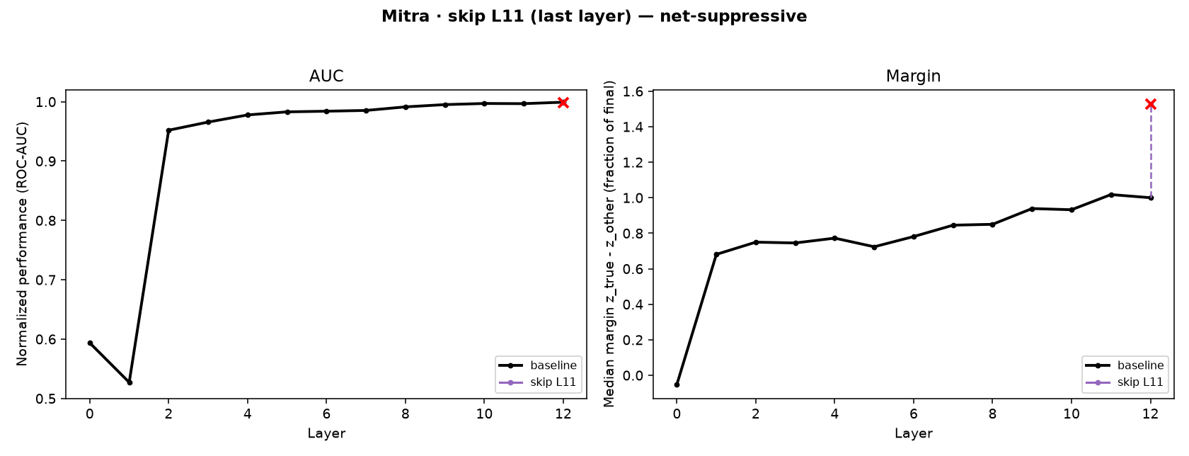 Figure 5: Mitra, skipping the final layer. ROC AUC does not move, whereas the logit margin indicates over-confidence.
Dip and recovery. Skipping layer 6 of Mitra also leaves ROC AUC flat, while the margin collapses from 0.85 to 0.36 and climbs back to 0.87 against a baseline of 0.97. This is the phenomenon of Section 3, invisible under ROC AUC.
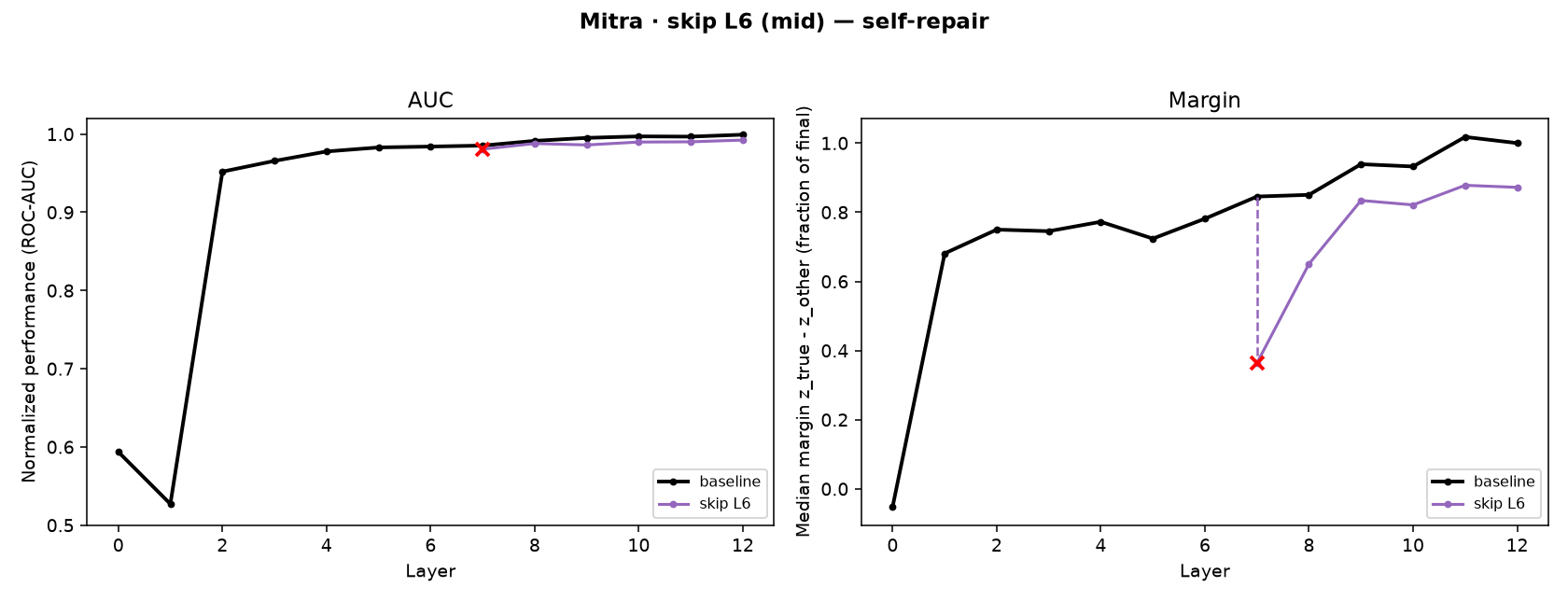 Figure 6: Mitra, skipping layer 6. ROC AUC rides the ceiling; the margin collapses to 0.36 and climbs back to 0.87.
5.3 Zero versus resample ablation
Next we provide empirical evidence for the advantages of resample ablation over zero ablation.
Magnitude. Zero ablation deletes a layer’s write, which leaves the residual stream with a norm the model never encounters.3 We measure the norm-preservation ratio, i.e., the norm of the residual after the ablation as a fraction of its clean norm, read at the decoded position. A faithful ablation should maintain it near \(1\).
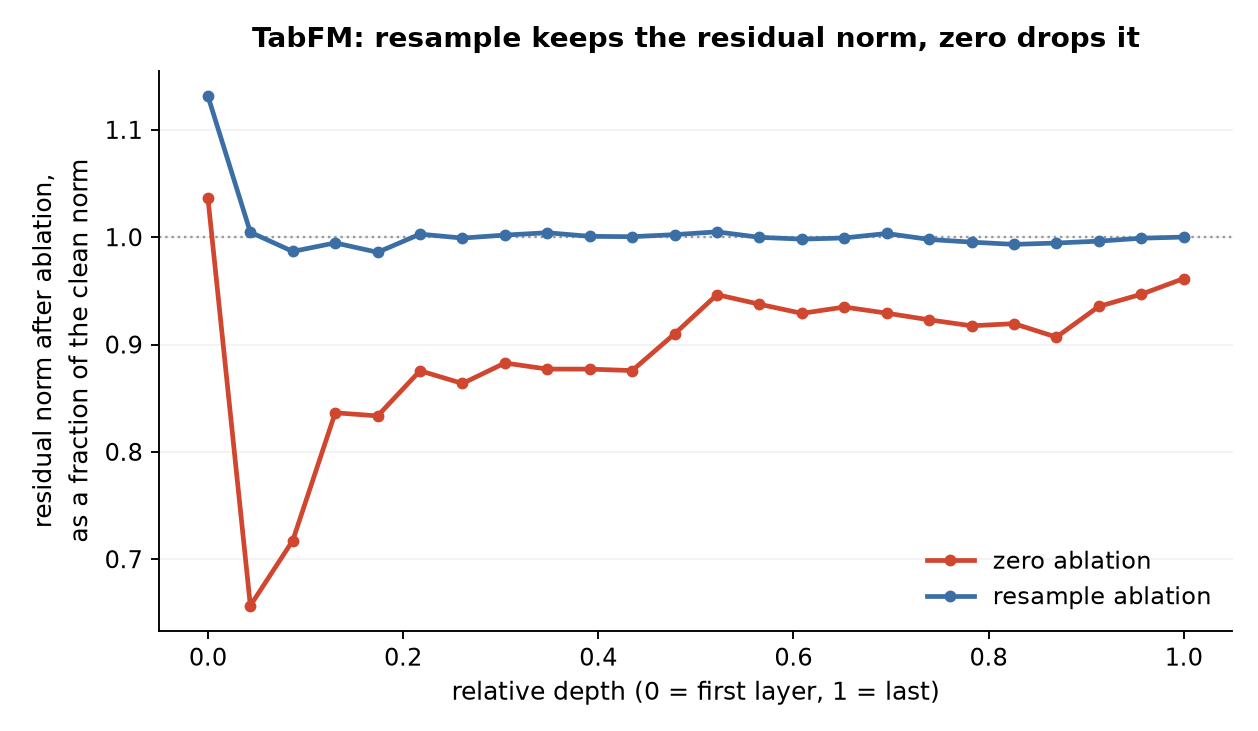 Figure 7: residual norm after ablation as a fraction of the clean norm, by relative depth. Resample ablation tracks \(1\) at every depth; zero ablation sits below it throughout. TabFM is shown here; the other three models are in Appendix B.
Across the four models the smallest ratio is \(0.96\) to \(1.00\) under resample ablation, against \(0.14\) to \(0.66\) under zero ablation.
Stability. A faithful ablation should also perturb consistently. The quantity to look at is the immediate drop: for an ablated layer \(m\), the loss of margin at the next depth,
\[\text{drop}(m) = \text{margin}^{\text{clean}}[m+1] - \text{margin}^{\text{ablated}}[m+1] .\]Since each ablation removes one layer’s contribution, the drop should be of a comparable size from layer to layer. A negative value means the ablation improved the margin, which a layer can genuinely cause if it suppresses the true class (e.g., the last layer of Mitra in Figure 5).
We measure two quantities: the standard deviation of the drop across layers, and the largest negative drop. A faithful ablation should keep both small. For the latter, a drop several times the clean final margin is not what one layer’s own contribution looks like: under zero ablation the residual norm has collapsed, and the LayerNorms downstream rescale by it, which amplifies whatever signal remains.
In Figure 8, we see that the standard deviation of the drop across layers is two to six times larger under zero ablation. Moreover, zero ablation produces negative drops of up to three times the clean final margin. Under resample ablation the largest negative drop is \(0.17\).
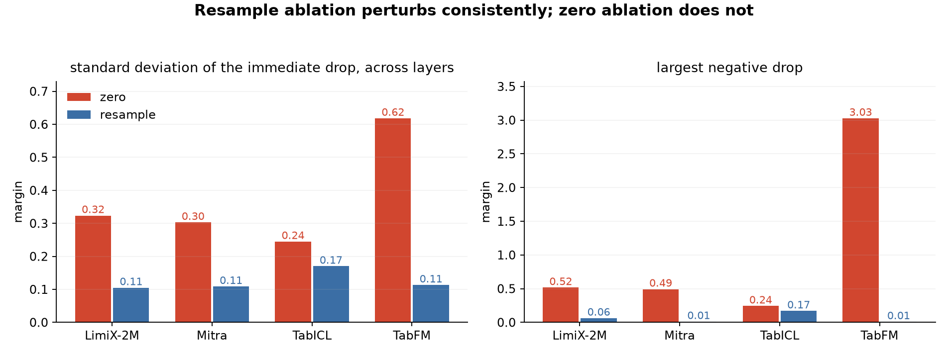 Figure 8: standard deviation of the immediate drop across the layers of each model (left) and the largest negative drop (right), margin coordinate. Per-model values are in Appendix B.
The phenomenon survives the change. The dip and recovery is present under both improvement and is easier to see (the trajectories are tighter and none of them crosses the clean baseline remarkably). An example is given in Figure 9 below.
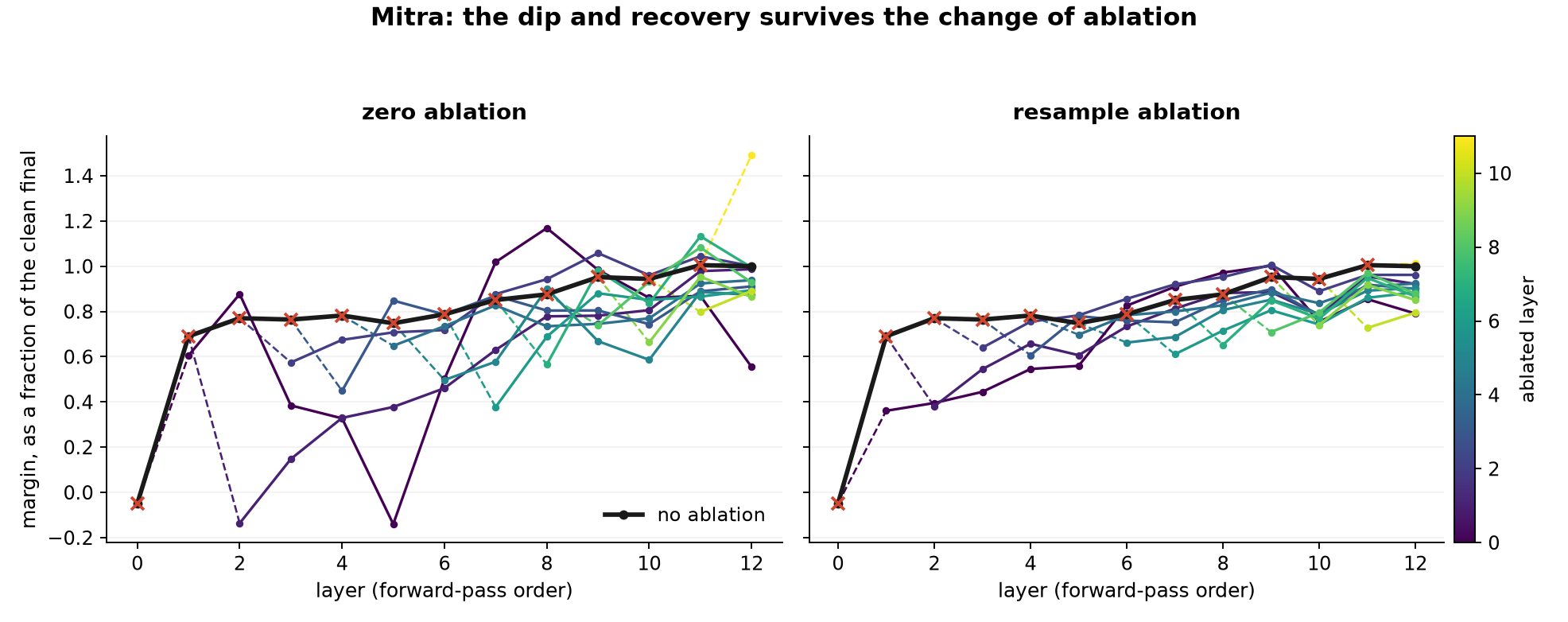 Figure 9: Mitra, every layer ablated in turn, under zero ablation (left) and resample ablation (right). Under zero the trajectories scatter and several cross the unablated baseline; under resample each ablated layer still dips at the next depth and then climbs back.
5.4 The compensation effect is approximately zero
We next answer the key question: whether self-repair is present in TFMs. We approach it via the two criteria (in Section 4.2): (i) qualitatively, that compensation is present at all, and (ii) quantitatively, that it is systematic rather than incidental.
Qualitatively. We plot the direct effect against the total effect, one point per (layer, task) pair. Figure 10 names the five regions of that plane. Three of them are the scenarios of Table 1. The plane adds two more: (i) indirectly important, where a layer writes no decision itself but is still needed by later layers, and (ii) amplified, where the downstream reaction enlarges the loss instead of absorbing it. The region we are looking for is repaired, below the diagonal.
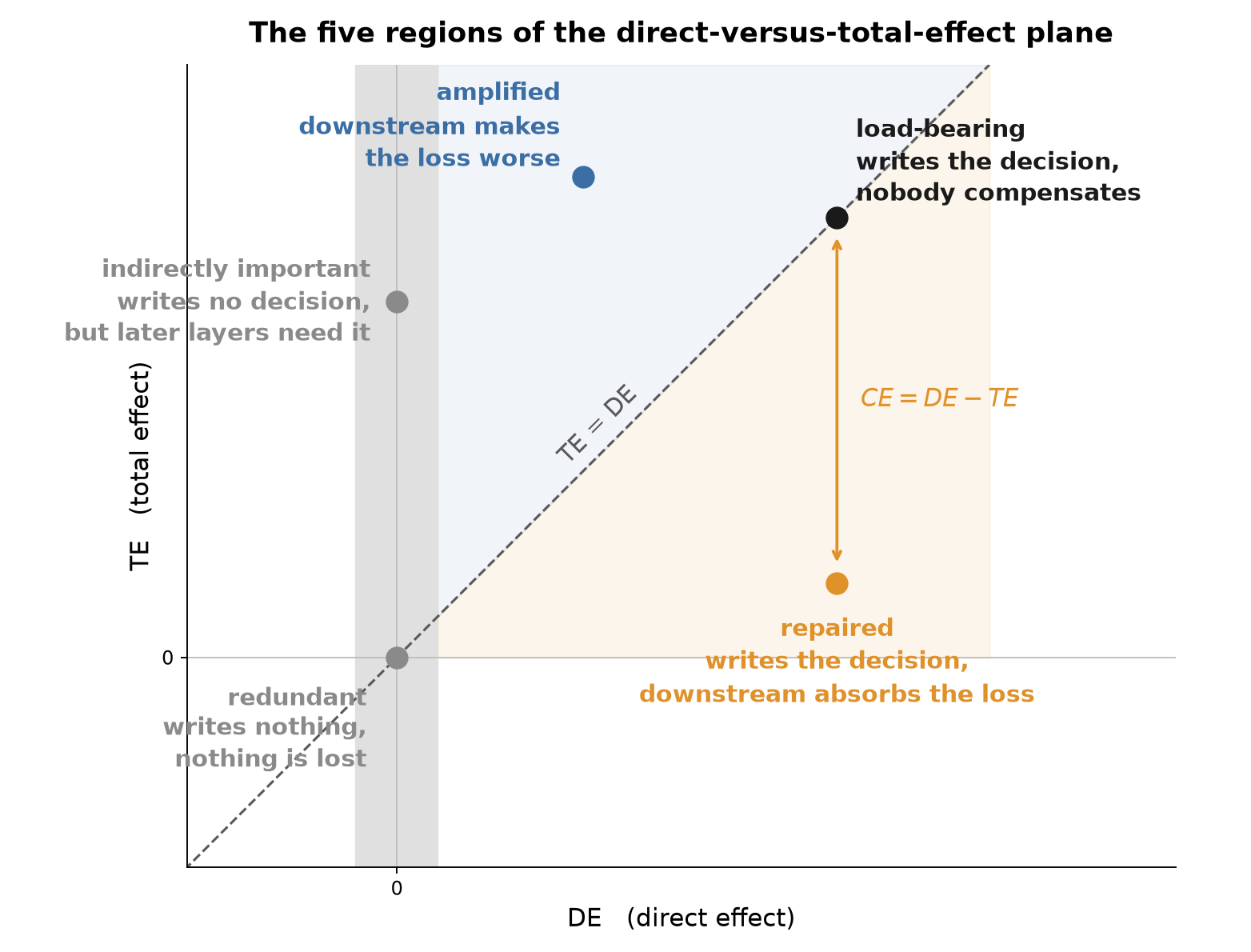 Figure 10: how to read Figure 11. The grey stripe is the band in which we treat the direct effect as zero, the dashed line is \(TE = DE\), i.e., no downstream reaction, and the vertical gap between a point and that line is the compensation effect.
Figure 11 is our main result.
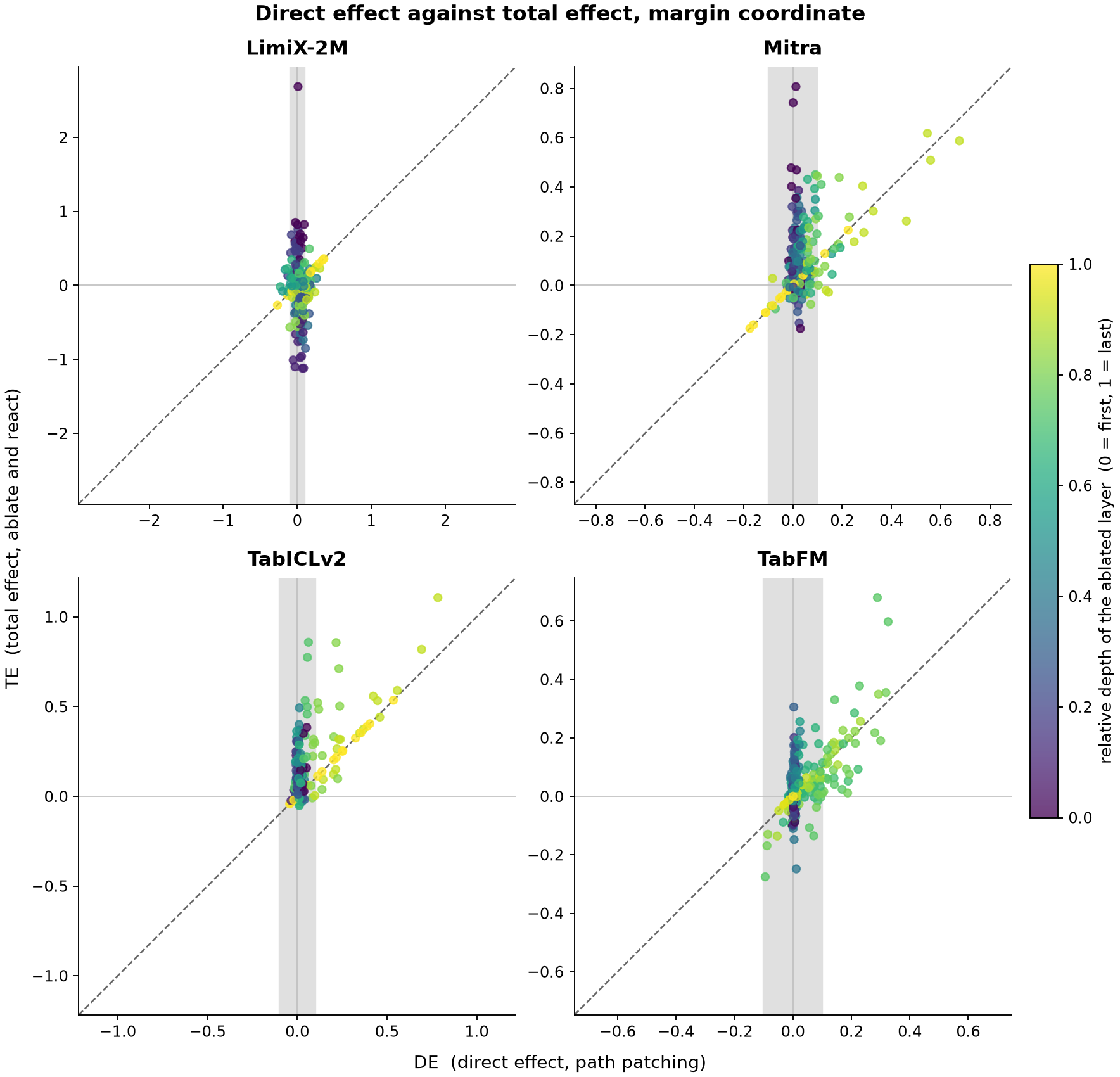 Figure 11: direct effect against total effect, margin coordinate, four TFMs. Colour is the relative depth of the ablated layer. The below-diagonal cloud in language models (Figure 2) is absent for TFMs.
We observe three things.
- The late layers of every model sit on the diagonal with \(DE > 0\): they write the decision directly and nothing compensates for them.
- The remaining layers form a vertical band at \(DE \approx 0\), which means most layers do not write the decision directly.
- The below-diagonal repair cloud of Figure 2 does not appear.
Figure 11 shows where the mass lies. We assign every point to one of the five regions of Figure 10, treating a direct effect within \(0.1\) of zero as zero.
| model | redundant | indirectly important | load-bearing | repaired | amplified | mean \(CE\) |
|---|---|---|---|---|---|---|
| LimiX-2M | 16% | 53% | 15% | 11% | 3% | \(+0.09\) |
| Mitra | 44% | 40% | 10% | 2% | 2% | \(+0.01\) |
| TabICL | 41% | 40% | 13% | 0% | 5% | \(-0.08\) |
| TabFM | 78% | 10% | 7% | 1% | 1% | \(+0.00\) |
Table 2: share of (layer, task) pairs in each region of Figure 11. The largest region of each model is in bold, together with any region within five points of it. The repaired region holds 0–11% in every model, and the mean compensation effect is within \(0.09\) of zero in all four.
Two observations follow.
- Repair is never the dominant region. It holds 0–11% of the points in every model. This is the quantitative form of the null, i.e., the hypothesis we are testing against, that the downstream layers do not compensate.
- Redundant and indirectly important carry the mass, 69–88% of the points taken together. TabFM is almost all redundancy (78%), whereas in LimiX-2M most such layers are indirectly important (53%).
LimiX-2M is the least favourable case for our conclusion: it has both the largest repaired share, 11%, and the largest mean compensation effect, \(+0.09\). A compensation effect of \(+0.09\) is 9% of the model’s own clean confidence. The second requirement of Section 4.2 fails as well, as we show next.
Quantitatively. Points below the diagonal say only that compensation sometimes happens. If it is a mechanism, it should also be regular: a layer that writes more of the decision should have more of it restored. This is the second thing we test, following the approach of [1].
- Fit: For a layer \(m\), the 15 tasks give 15 pairs \((DE, CE)\), one per task. And we fit a line \(CE = a + b \cdot DE\) to them.
- Read: The slope \(b\) is the share of the direct contribution that the downstream layers restore and the remaining \(1-b\) survives to the output as damage. The \(R^2\) of the fit, i.e., the share of the variation in \(CE\) that the line accounts for, says how reliably that share holds across tasks.
- Criterion: if layers truly compensate, we should observe a high \(R^2\) with a slope in \((0, 1)\) at some layers. For example, in the language model studied in [1], we get \(R^2 = 0.92\) and slope \(0.69\) at layer 23 (Figures 4b and 4d of [1]).
We fit every layer of every model and report the one where \(R^2\) peaks, i.e., the tightest relation in each model. For a binary task our margin is, up to a factor of two, the centred logit read in [1], so the comparison is on comparable ground. Table 3 and Figure 12 summarize our findings.
| model | apex layer | slope | \(R^2\) |
|---|---|---|---|
| LimiX-2M | L10 | \(-0.03\) | 0.00 |
| Mitra | L10 | \(+0.08\) | 0.04 |
| TabICL | L10 | \(-0.41\) | 0.58 |
| TabFM | L18 | \(-0.08\) | 0.04 |
| Chinchilla 7B [1] | L23 | \(+0.69\) | 0.92 |
Table 3: per-layer regression of \(CE\) on \(DE\) across the 15 tasks, reported at the layer where \(R^2\) peaks. The last row is the language-model reference. No TFM layer combines a high \(R^2\) with a slope in \((0, 1)\).
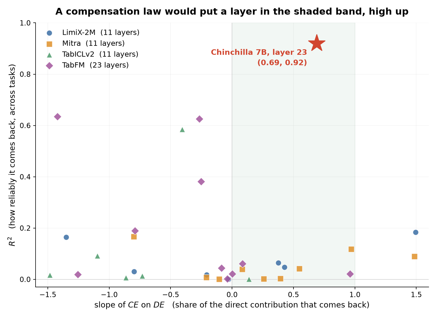 Figure 12: one point per layer per model (excluding last layer because \(CE = 0\)). The shaded band corresponds to a slope in \((0, 1)\), i.e., the downstream layers restore part of what the layer writes. A compensation law would put a layer inside the band and high u, i.e., \(R^2\) is large. The language-model reference point is shown as a red star.
No layer falls inside the band with a high \(R^2\). The closest any layer comes is TabICL L10, at \(R^2 = 0.58\), but its slope is negative, \(-0.41\), so the larger the direct contribution, the more the downstream layers enlarge its loss. We therefore find no sign of a compensation law in any of the four models.
In Appendix C we redo the analysis row by row, and on a model with a linear output head. The answer does not change.
6. Conclusion
We measure self-repair as the gap between a component’s direct and total effect. Across four TFMs and 15 tasks that gap is approximately zero, and the compensation law of language models holds at no layer. The recovery reported for TFMs is passive redundancy, not active compensation.
Our work opens interesting future directions:
- Finer resolution. Ablating a whole layer may hide individual heads that do compensate. Can we find a head that self-repairs?
- Other models. LimiX-16M and the TabPFN family, for which Balef et al. [5] report the clearest self-repair, are not covered here.
- The mechanism of redundancy. Is a lost feature recomputed on demand from the input table, which stays in context, or is it already copied along the residual stream?
7. Reproducibility
All code used in this paper are available in the tfmlens repository.
Acknowledgement. We thank Martin Veron for the discussion and feedback on the write-up. The experiments and the write-up were carried out with the assistance of Claude Code.
References
[1] T. McGrath, M. Rahtz, J. Kramar, V. Mikulik, S. Legg. The Hydra Effect: Emergent Self-repair in Language Model Computations. arXiv:2307.15771, 2023.
[2] K. Wang, A. Variengien, A. Conmy, B. Shlegeris, J. Steinhardt. Interpretability in the Wild: a Circuit for Indirect Object Identification in GPT-2 small. arXiv:2211.00593, 2022.
[3] C. Rushing, N. Nanda. Explorations of Self-Repair in Language Models. arXiv:2402.15390, 2024.
[4] J. Miller, B. Chughtai, L. Sharkey. Transformer Circuit Faithfulness Metrics are not Robust. arXiv:2407.08734, 2024.
[5] A. R. Balef, M. Koshil, K. Eggensperger. Is One Layer Enough? Understanding Inference Dynamics in Tabular Foundation Models. arXiv:2605.06510, 2026.
[6] J. Pearl. Direct and Indirect Effects. Proceedings of the 17th Conference on Uncertainty in Artificial Intelligence (UAI), 2001.
[7] F. Zhang, N. Nanda. Towards Best Practices of Activation Patching in Language Models: Metrics and Methods. arXiv:2309.16042, 2024.
Appendix A: the layer-skipping experiment on all four models
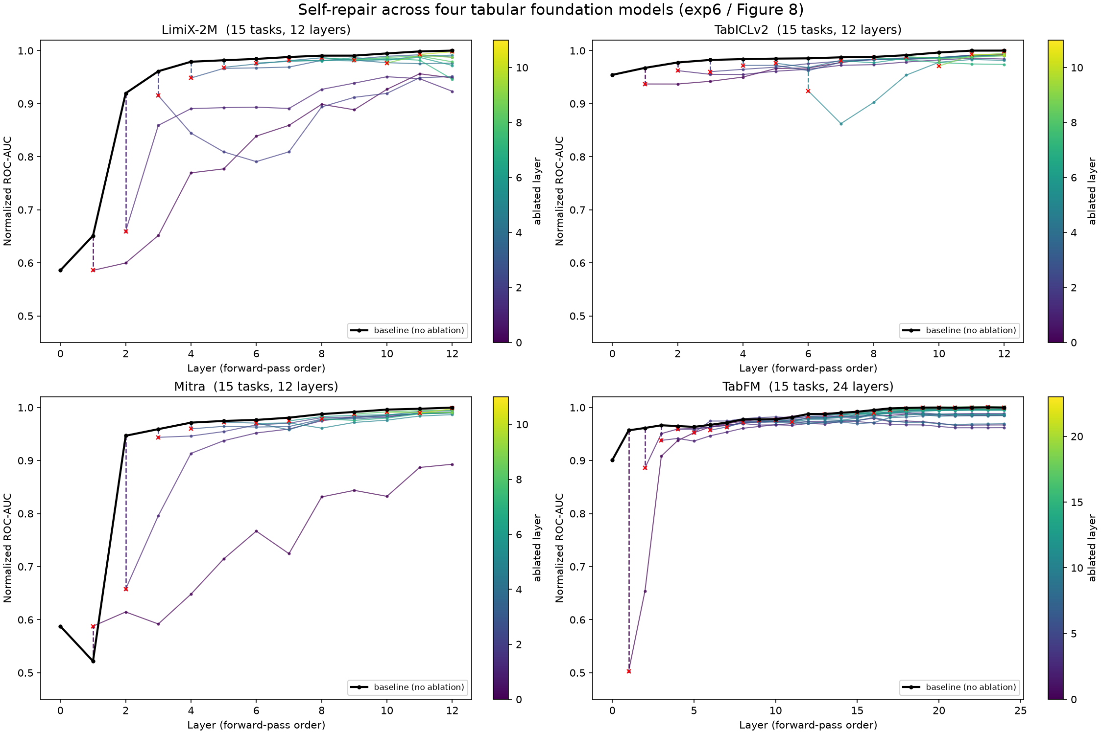 Figure 13: our reproduction of the layer-skipping experiment of Balef et al. [5] on four TFMs, 15 tasks each. Black is the unablated baseline; each coloured curve skips one layer, marked by a red cross. The right panel of Figure 3 is the LimiX-2M panel of this figure.
Appendix B: ablation diagnostics on all four models
| model | min norm ratio, zero / resample | std of the immediate drop | largest negative drop |
|---|---|---|---|
| LimiX-2M | 0.14 / 1.00 | 0.32 / 0.11 | 0.52 / 0.06 |
| Mitra | 0.52 / 1.00 | 0.30 / 0.11 | 0.49 / 0.01 |
| TabICL | 0.64 / 0.96 | 0.24 / 0.17 | 0.24 / 0.17 |
| TabFM | 0.66 / 0.99 | 0.62 / 0.11 | 3.03 / 0.01 |
Table 4: the two ablation operators compared, zero / resample in each cell. TabFM is the extreme case: under zero ablation one layer’s removal improves the margin by three times its clean final value.
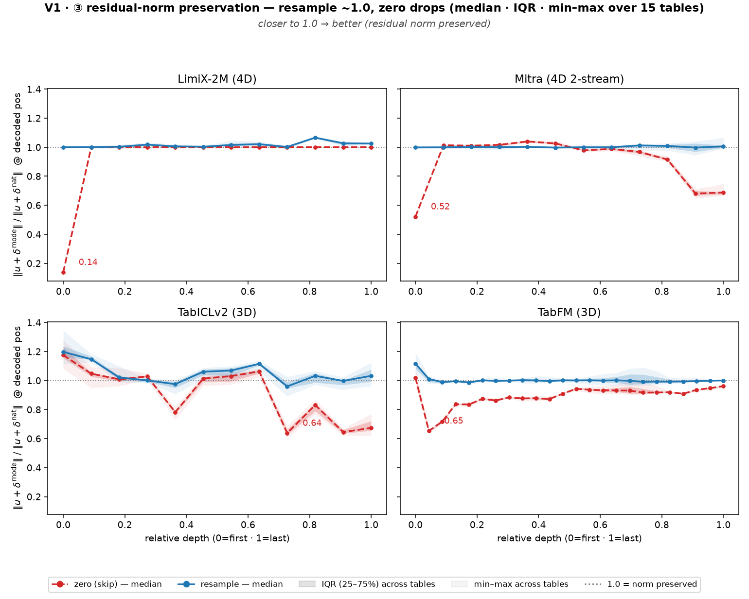 Figure 14: residual norm after ablation as a fraction of the clean norm, all four models, by relative depth. Lines are the median over the 15 tasks; bands are the interquartile range and the range across tasks. Figure 7 is the TabFM panel.
Matched magnitude is not on its own enough: a substitute of the right size pointing in a direction the model never uses is still a shock. We therefore also compare directions. Let \(c_{\text{cross}}\) be the cosine between the source write and the native write it replaces, and \(c_{\text{within}}\) the cosine between two native writes from different rows of the same table, which is the yardstick for how aligned genuine writes already are.
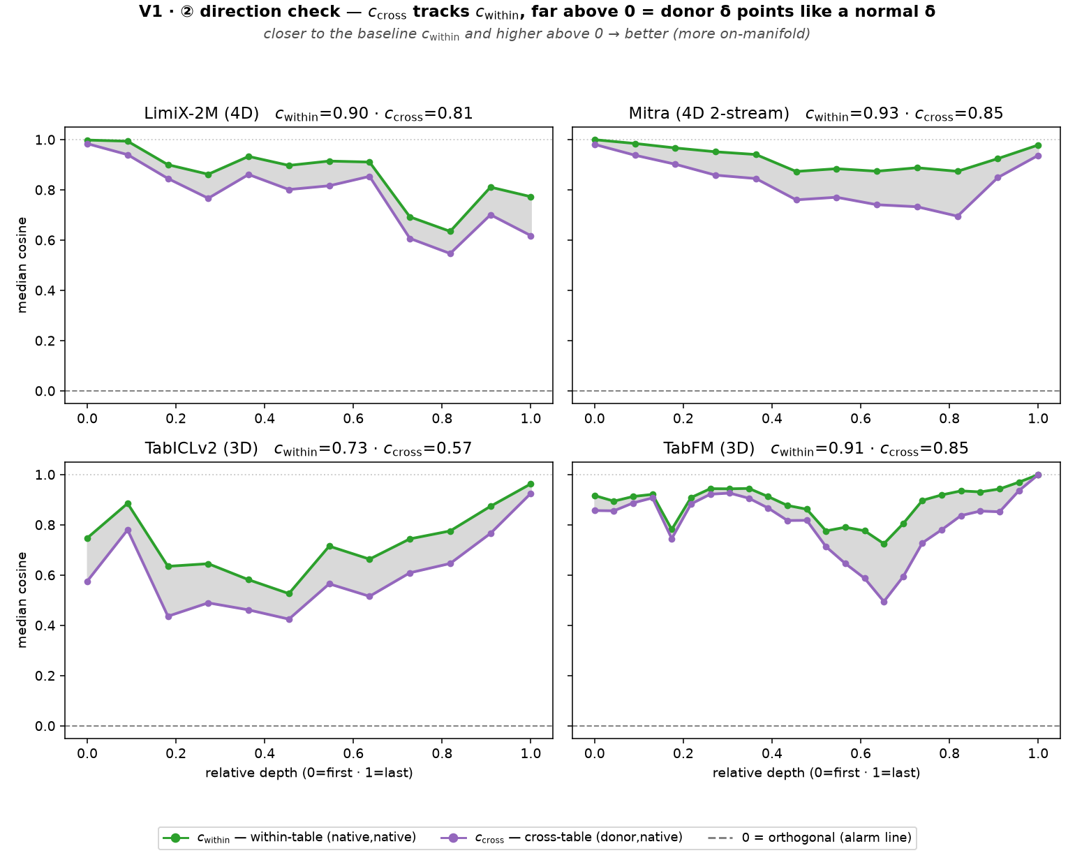 Figure 15: cosine between the source write and the write it replaces (cross), against the cosine between two native writes (within), all four models.
| model | \(c_{\text{within}}\) | \(c_{\text{cross}}\) |
|---|---|---|
| LimiX-2M | 0.85 | 0.77 |
| Mitra | 0.93 | 0.83 |
| TabICL | 0.71 | 0.58 |
| TabFM | 0.87 | 0.80 |
Table 5: direction of the substituted write. In every model \(c_{\text{cross}}\) tracks \(c_{\text{within}}\) and stays well above zero, i.e., the source write points where native writes point. TabICL’s writes are less aligned to begin with, and its \(c_{\text{cross}}\) is lower in proportion.
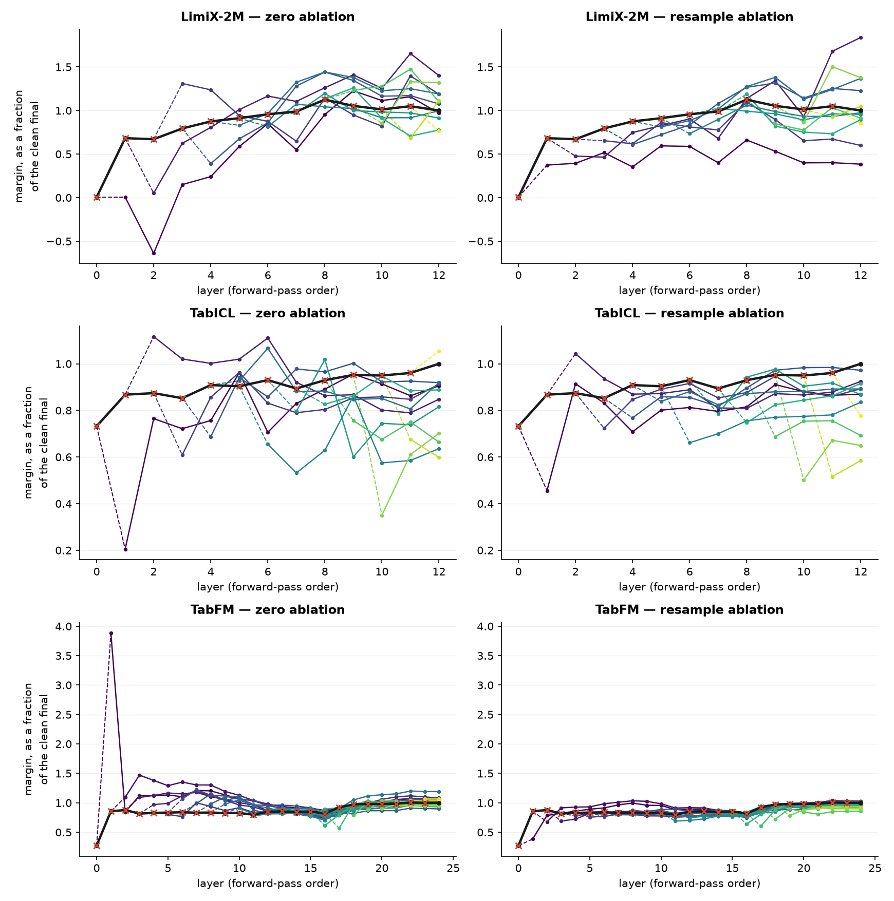 Figure 16: LimiX-2M, TabICL and TabFM, every layer ablated in turn, under zero ablation (left column) and resample ablation (right column). Figure 9 is the Mitra case. TabFM under zero ablation is the extreme: one ablated layer improves the margin by three times its clean final value, sending it to almost four times that value.
Appendix C: two further checks on the compensation effect
Two checks beyond the compensation law of Section 5.4: one at a finer resolution, one against a possible artifact of the readout.
Per-row de-aggregation. Each point in Figure 11 aggregates roughly 500 query rows, so a mean of zero is compatible with cancellation between rows of opposite sign, or with strong repair confined to a small subpopulation. We therefore de-aggregate and inspect the distribution of \(CE\) over individual rows.
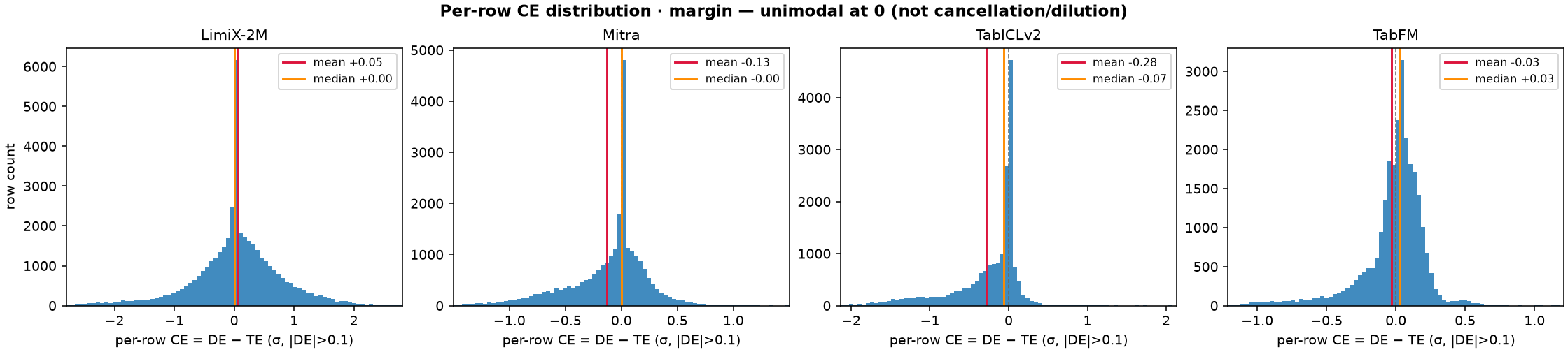 Figure 17: distribution of the per-row compensation effect. All four models are unimodal at zero.
The per-row distributions are unimodal at zero in all four models, neither bimodal nor right-skewed, which rules out both alternatives. Restricting to rows whose direct effect exceeds \(0.1\) standard deviations, the share of rows with \(CE > 0\) ranges from 23% to 58% across models, so no model sits systematically on the repair side. The only signal stable across tasks is negative \(CE\) in TabICL, i.e., amplification, which is the opposite of repair.
Not an artifact of the readout. Mitra serves as an anchor. Its head is linear, so \(TE = DE + IE\) holds with zero residual and the decomposition is exact. Mitra shows \(CE = +0.01\), i.e., the null is not produced by nonlinearity in the decoder or by LayerNorm rescaling.
-
The two numbers carry distinct information. The \(R^2\) says the compensation is systematic, i.e., how much is lost predicts how much is restored. The slope says it is partial, i.e., about 70% of the direct contribution is restored and the remaining 30% survives to the output. ↩
-
Some models keep one position per cell, i.e., one for each feature of a row together with a label position that the decoder reads. There we match these two kinds as well, drawing feature positions from feature positions and the label position from label positions. Models that represent a row by a single vector have no such axis. ↩
-
The norm matters because every LayerNorm downstream of the ablated layer, including the one in the decoder, rescales by it, so a residual of an unfamiliar size is read in a regime the model was never trained on. ↩
