Motivation

In this project, I implemented the algorithm in Deep Structural Network Embedding (KDD 2016) using Keras

The algorithm in the paper actually blew my mind because:

it uses auto-encoder for representation learning in an interesting way
the experiment result really demonstrates its superiority

To see how it works in reality, I set out to implement it by myself.

During the process, I gained some hand-on experience on:

Keras’s basics, defining custom loss function, defining custom callback, auto-encoder basics and implementing it in keras
hyper-parameter tuning: grid search
tensorboard visualization/exploration, one good example
the code is hosted in github

The algorithm

I describe the algorithm very briefly. For more details, I recommend reading the papers

Firstly, the algorithm’s goal is to learn low dimensional embedding for each node.

Then for this goal, the loss function captures two aspects:

neighboring nodes should have embeddings close to each other (“1st order proximity” referred in the paper)
each node’s embedding should be able to predict its neighboring nodes (“2nd order proximity” referred in the paper )

The auto-encoder comes into play for 2nd order proximity.

The algorithm implemented in Keras

First, we define the loss functions in the paper:

import math
import networkx as nx
import numpy as np
from functools import reduce

import keras
from keras import Model, backend as K, regularizers
from keras.layers import Dense, Embedding, Input, Reshape, Subtract, Lambda


def build_reconstruction_loss(beta):
    """
    return the loss function for 2nd order proximity

    beta: the definition below Equation 3"""
    assert beta > 1

    def reconstruction_loss(true_y, pred_y):
        diff = K.square(true_y - pred_y)

        # borrowed from https://github.com/suanrong/SDNE/blob/master/model/sdne.py#L93
        weight = true_y * (beta - 1) + 1

        weighted_diff = diff * weight
        return K.mean(K.sum(weighted_diff, axis=1))  # mean square error
    return reconstruction_loss


def edge_wise_loss(true_y, embedding_diff):
    """1st order proximity
    """
    # true_y supposed to be None
    # we don't use it
    return K.mean(K.sum(K.square(embedding_diff), axis=1))  # mean square error

Then the main algorithm

class SDNE():
    def __init__(self,
                 graph,
                 encode_dim,
                 weight='weight',
                 encoding_layer_dims=[],
                 beta=2, alpha=2,
                 l2_param=0.01):
        """graph: nx.Graph
        encode_dim: int, length of inner most dim
        beta: beta parameter under Equation 3
        alpha: weight of loss function on self.edges
        """
        self.encode_dim = encode_dim

        ###################
        # GRAPH STUFF
        ###################

        self.graph = graph
        self.N = graph.number_of_nodes()
        self.adj_mat = nx.adjacency_matrix(self.graph).toarray()
        self.edges = np.array(list(self.graph.edges_iter()))

        # weights
        # default to 1
        weights = [graph[u][v].get(weight, 1.0)
                   for u, v in self.graph.edges_iter()]
        self.weights = np.array(weights, dtype=np.float32)[:, None]

        if len(self.weights) == self.weights.sum():
            print('the graph is unweighted')
        
        ####################
        # INPUT
        ####################

        # one end of an edge
        input_a = Input(shape=(1,), name='input-a', dtype='int32')
        # the other end of an edge
        input_b = Input(shape=(1,), name='input-b', dtype='int32')
        edge_weight = Input(shape=(1,), name='edge_weight', dtype='float32')

        ####################
        # network architecture
        ####################
        encoding_layers = []
        decoding_layers = []
        
        embedding_layer = Embedding(output_dim=self.N, input_dim=self.N,
                                    trainable=False, input_length=1, name='nbr-table')
        # if you don't do this, the next step won't work
        embedding_layer.build((None,))
        embedding_layer.set_weights([self.adj_mat])
        
        encoding_layers.append(embedding_layer)
        encoding_layers.append(Reshape((self.N,)))
        
        # encoding
        encoding_layer_dims = [encode_dim]

        for i, dim in enumerate(encoding_layer_dims):
            layer = Dense(dim, activation='sigmoid',
                          kernel_regularizer=regularizers.l2(l2_param),
                          name='encoding-layer-{}'.format(i))
            encoding_layers.append(layer)

        # decoding
        decoding_layer_dims = encoding_layer_dims[::-1][1:] + [self.N]
        for i, dim in enumerate(decoding_layer_dims):
            if i == len(decoding_layer_dims) - 1:
                activation = 'sigmoid'
            else:
                # activation = 'relu'
                activation = 'sigmoid'
            layer = Dense(
                dim, activation=activation,
                kernel_regularizer=regularizers.l2(l2_param),
                name='decoding-layer-{}'.format(i))
            decoding_layers.append(layer)
        
        all_layers = encoding_layers + decoding_layers

        ####################
        # VARIABLES
        ####################
        encoded_a = reduce(lambda arg, f: f(arg), encoding_layers, input_a)
        encoded_b = reduce(lambda arg, f: f(arg), encoding_layers, input_b)

        decoded_a = reduce(lambda arg, f: f(arg), all_layers, input_a)
        decoded_b = reduce(lambda arg, f: f(arg), all_layers, input_b)
        
        embedding_diff = Subtract()([encoded_a, encoded_b])

        # add weight to diff
        embedding_diff = Lambda(lambda x: x * edge_weight)(embedding_diff)

        ####################
        # MODEL
        ####################
        self.model = Model([input_a, input_b, edge_weight],
                           [decoded_a, decoded_b, embedding_diff])
        
        reconstruction_loss = build_reconstruction_loss(beta)

        self.model.compile(
	    optimizer='adadelta',
            loss=[reconstruction_loss, reconstruction_loss, edge_wise_loss],
            loss_weights=[1, 1, alpha])
                           
        self.encoder = Model(input_a, encoded_a)

        # for pre-training
        self.decoder = Model(input_a, decoded_a)
        self.decoder.compile(optimizer='adadelta',
                             loss=reconstruction_loss)

    def pretrain(self, **kwargs):
        """pre-train the autoencoder without edges"""
        nodes = np.arange(self.graph.number_of_nodes())
        node_neighbors = self.adj_mat[nodes]
                
        self.decoder.fit(nodes[:, None],
                         node_neighbors,
                         shuffle=True,
                         **kwargs)

    def train_data_generator(self, batch_size=32):
        # this can become quadratic if using dense
        m = self.graph.number_of_edges()
        while True:
            for i in range(math.ceil(m / batch_size)):
                sel = slice(i*batch_size, (i+1)*batch_size)
                nodes_a = self.edges[sel, 0][:, None]
                nodes_b = self.edges[sel, 1][:, None]
                weights = self.weights[sel]
                
                neighbors_a = self.adj_mat[nodes_a.flatten()]
                neighbors_b = self.adj_mat[nodes_b.flatten()]

                # requires to have the same shape as embedding_diff
                dummy_output = np.zeros((nodes_a.shape[0], self.encode_dim))

                yield ([nodes_a, nodes_b, weights],
                       [neighbors_a, neighbors_b, dummy_output])

    def fit(self, log=False, **kwargs):
        """kwargs: keyword arguments passed to `model.fit`"""
        if log:
            callbacks = [keras.callbacks.TensorBoard(
                log_dir='./log', histogram_freq=0,
                write_graph=True, write_images=False)]
        else:
            callbacks = []

        callbacks += kwargs.get('callbacks', [])
        if 'callbacks' in kwargs:
            del kwargs['callbacks']

        if 'batch_size' in kwargs:
            batch_size = kwargs['batch_size']
            del kwargs['batch_size']
            gen = self.train_data_generator(batch_size=batch_size)
        else:
            gen = self.train_data_generator()

        self.model.fit_generator(
            gen,
            shuffle=True,
            callbacks=callbacks,
            pickle_safe=True,
            **kwargs)
        
    def get_node_embedding(self):
        """return the node embeddings as 2D array, #nodes x dimension"""
        nodes = np.array(self.graph.nodes())[:, None]
        return self.encoder.predict(nodes)

    def save(self, path):
        self.model.save(path)

Hyperparameter tuning

I found that in practice, grid search is an effective way to gain intuition on setting the hyper parameters.

The following code snippets demonstrates how to do this (For more complete example, please refer here)

# we define the parameter values to try
parameter_grid = {'alpha': [1, 10,],
                  'l2_param': [1e-3, 1e-4, 1e-5],
                  'pretrain_epochs': [0, 5, 10],
                  'epochs': [10, 50, 100]}

parameter_values = list(product(*parameter_grid.values()))
parameter_keys = list(parameter_grid.keys())

parameter_dicts = [dict(list(zip(parameter_keys, values))) for values in parameter_values]


def one_run(params):
    alpha = params['alpha']
    l2_param = params['l2_param']
    pretrain_epochs = params['pretrain_epochs']
    epochs = params['epochs']

    model = SDNE(g, encode_dim=100, encoding_layer_dims=[1720, 200],
                 beta=2,
                 alpha=alpha,
                 l2_param=l2_param)
    model.pretrain(epochs=pretrain_epochs, batch_size=32)

    n_batches = math.ceil(g.number_of_edges() / batch_size)

    model.fit(epochs=epochs, log=True, batch_size=batch_size,
              steps_per_epoch=n_batches)

Then we run the training with each configuration

result = [one_run(g, dev_edges, test_edges, params)
          for params in tqdm(parameter_dicts)]

# dump to result some where
pkl.dump(result, open('outputs/{somewhere}.pkl', 'wb'))

In reality, I that setting training epochs to a large number is important. Because In many cases, I’m just too eager to see the result that I set the training epochs to a small number.

Experiments

embedding visualization on 20newsgroups

This dataset is directly available from sklearn.

Using the grid search method, the final hyper parameter I decided to use are:

l2_param=1e-3
alpha=2
epochs=1: I found larger training epochs outfits the data
without pre-training (as it does not seem to play an important role)

I selected the 3 classes as the same in the paper.

You can play with the embedding using tensorboard

An example is:

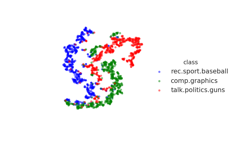
Unfortunately, I cannot reproduce the very separated clusters described in the paper.

However, you can try to train the embedding by yourself.

link prediction on grqc dataset

In this task, we hide some edges of the graph for validation and test and train the embedding using the remaining the edges.

The hyperparameters are:

l2_param=1e-3
alpha=2
epochs=200

Performance is reported in terms of precision@k.

Performance over epochs on validation data:

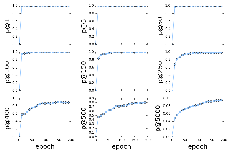
Using the above, I decided to terminate the training after 200 epochs, The performance for the test data is

p@1: 1.0
p@5: 1.0
p@50: 1.0
p@100: 1.0
p@150: 1.0
p@250: 0.996
p@400: 0.995
p@500: 0.976
p@5000: 0.1448

(Note that the k values we use here are half of the k values used in the paper. This is because the paper states that the grqc data contains 28980 edges however, the graph actually has 14490 edges (half!). So I divided the k values by 2)

visualizing Stackexchange tags

Out of curiosity, I created a dataset of the tags at Stackexchange datascience.

The dataset is created as follows:

download the data using data.stackexchange.com
extract the labels of each question
build the cooccurence graph using coconut (a tool created by me): frequency is normalized by log function

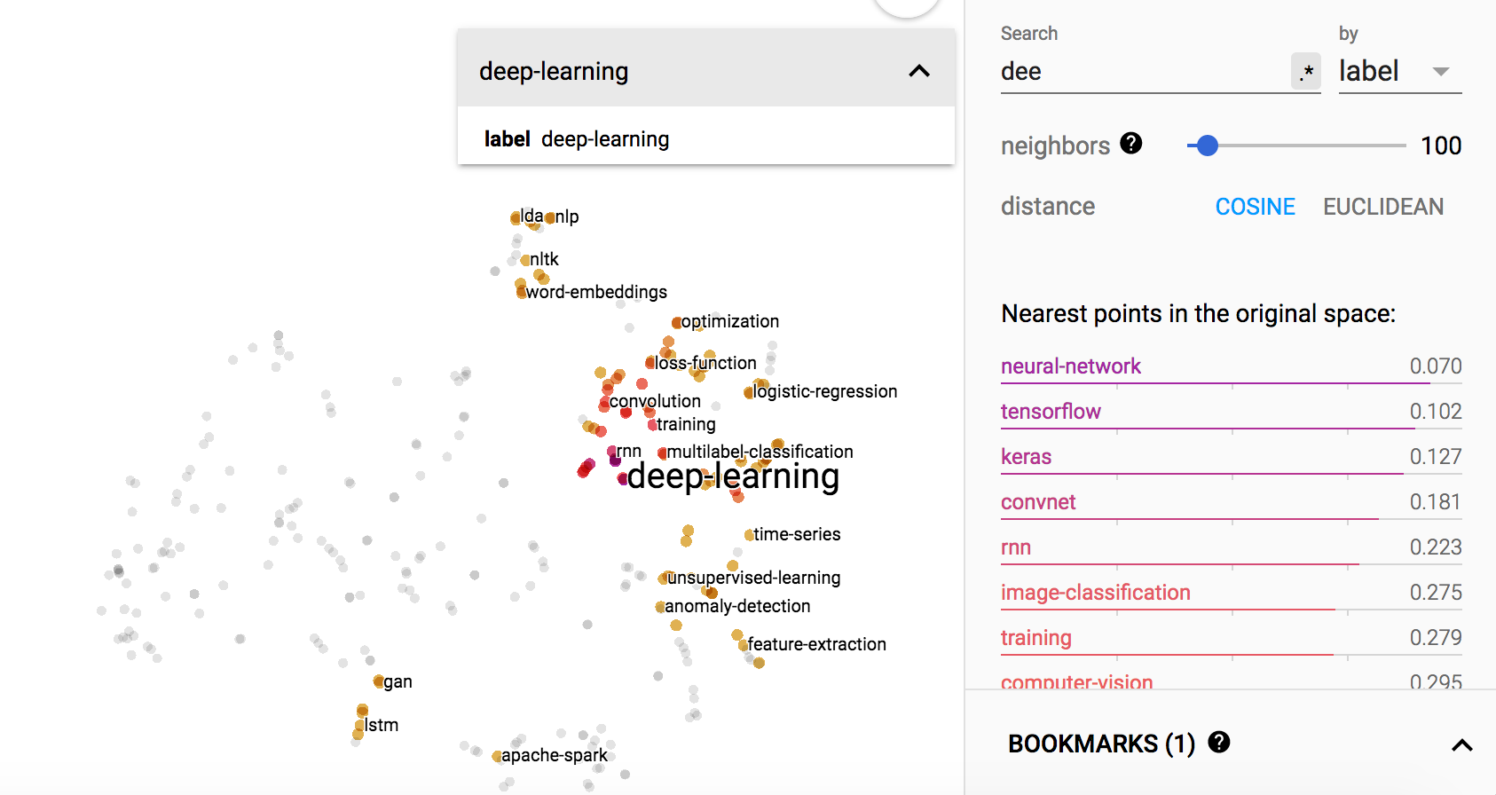
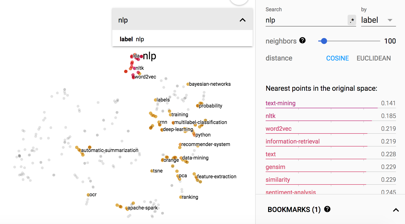
You can also play with the embedding using tensorboard

Some examples of the visualizations are:

“deep-learning”

“nlp”

“search-engine”