Interesting representations and where to find them

My solution to BlueDot Impact’s first Technical AI Safety Puzzle — a small but delightful interpretability challenge about how a neural net represents features. (Cover art generated with leonardo.ai.)
Earlier this year I took part in this puzzle. My submission did not win, but I enjoyed the exploration enough that I wanted to write it up.
This post is a fairly complete transcription of my solution. For the full details (extra plots, code snippets, and derivations) see the original write-up and the source code at xiaohan2012/bluedot-tais-puzzle. The puzzle’s own starter notebook (the trained model we were handed) lives at SamDower/bluedot-tais-puzzle.
Table of contents
- Table of contents
- The puzzle
- Q1 — The
countryfeature is not linearly separable - Q2 —
countrylives on a quadratic surface - Q3 — Building more interesting representations
- Takeaways
The puzzle
We are given a model that reads a short piece of text and predicts eight binary features at once — things like is this a question?, does it mention a person?, does it mention a country?. Internally the text runs through a sentence encoder and a small MLP head; the eight predictions are read off the final layer.
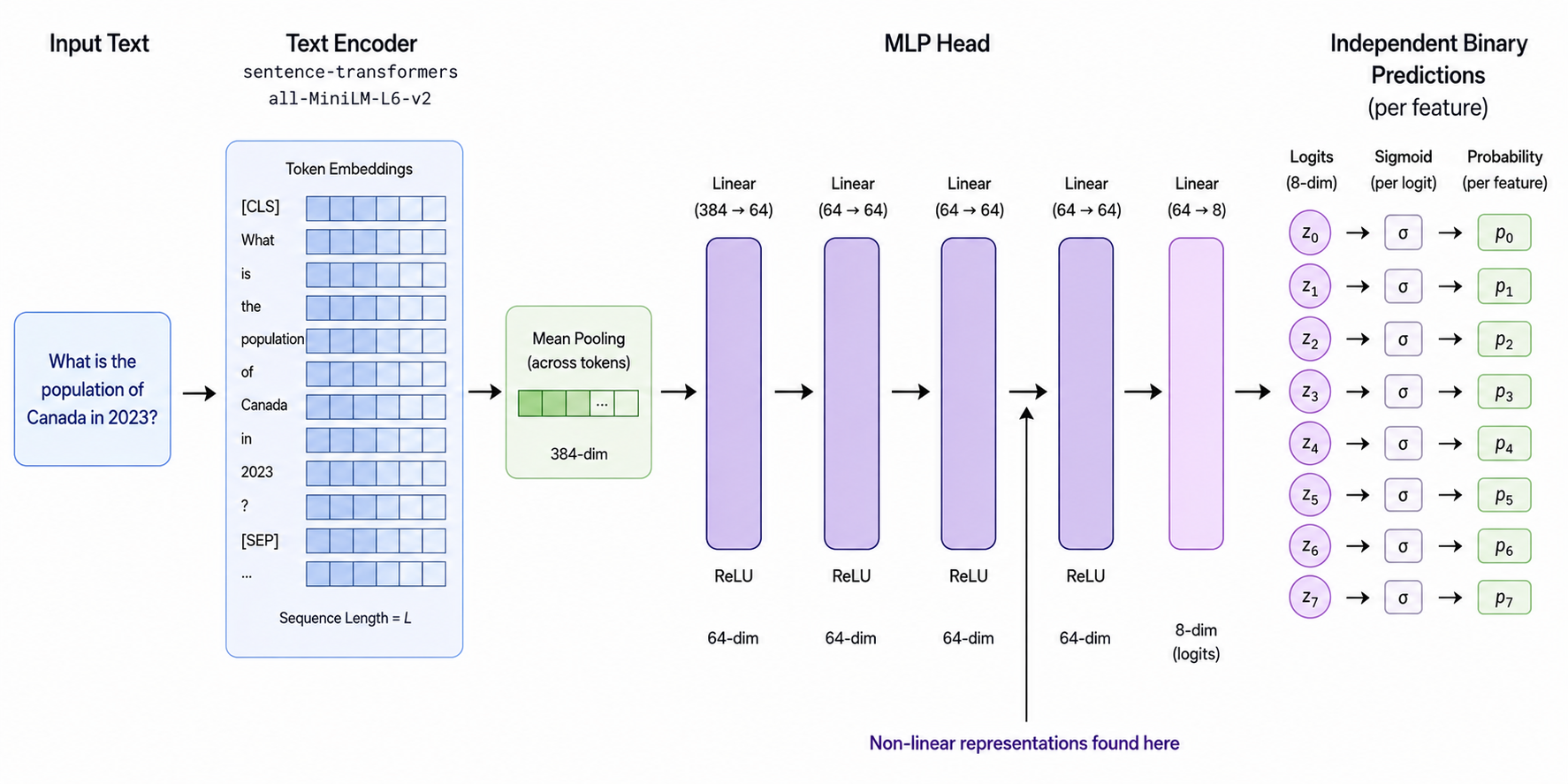
The given model: a all-MiniLM-L6-v2 encoder with mean pooling, feeding a 5-layer MLP head that outputs 8 independent binary predictions. The puzzle concerns the representations at hidden layer 2.
The interesting twist: at a specified layer, seven of the eight features are represented linearly — a single direction in activation space tells you the feature — but one feature is not. The puzzle has three parts:
- Identify which feature is not linearly represented.
- Explain the geometric structure the model uses for it.
- Invent a model that encodes some feature in a more interesting way — with “more interesting” being ours to define and defend.
The rest of this post follows those three tasks.
Q1 — The country feature is not linearly separable
The feature represented non-linearly at hidden layer 2 is country.
The detection method is straightforward:
- For each feature, fit a linear probe (logistic regression) on the training activations.
- Report its accuracy on the test set.
If a single direction encodes the feature, a linear probe should nail it. Here is what we get:
Table 1: Per-feature test accuracy of linear probes on hidden-layer-2 activations. country stands out as near chance-level.
| Feature | Test accuracy |
|---|---|
| number | 0.975 |
| question | 1.000 |
| color | 0.971 |
| food | 0.985 |
| sentiment | 0.982 |
| country | 0.427 |
| person | 0.998 |
| body_part | 0.980 |
Every feature except country is essentially perfectly decodable by a line; country sits at chance.
To complement the accuracy numbers, we can look at the distribution of the probe’s predicted log-odds per class. For a linearly separable feature (person) the two classes form well-separated bi-modal peaks; for country the two classes are completely mixed.
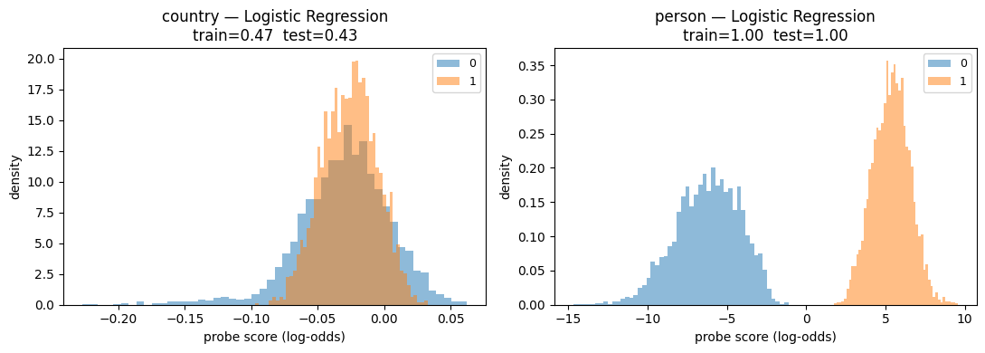
Figure 1: Per-class log-odds from the linear probe. country (left) is fully mixed; person (right) is cleanly bi-modal.
As we will see next, a more expressive probe pulls the country distributions apart.
Q2 — country lives on a quadratic surface
It turns out country can be separated by a quadratic surface (an ellipse-like boundary).
To build intuition, we project the hidden-layer-2 activations to 2D with PCA (the top two components explain ~78% of the variance). Coloring by country reveals a “sandwich”: one class is wrapped between two slabs of the other. No straight line separates them, but a curved boundary does.
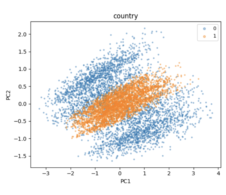
Figure 2: 2D PCA projection of hidden-layer-2 activations, colored by country. The sandwich shape hints at quadratic separability.
We can verify this by swapping the linear probe for a quadratic one. The only change is adding second-degree feature interactions; in scikit-learn:
make_pipeline(
    PolynomialFeatures(degree=2, include_bias=False),  # drop this and it reduces to a linear probe
    LogisticRegression(),
)
With this probe, test accuracy on country jumps from 0.427 to 0.931. The log-odds distribution confirms it — the degree-2 probe splits the two classes into clean bi-modal peaks, while the linear probe stays mixed.
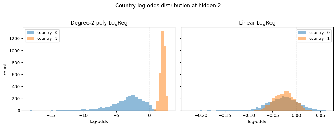
Figure 3: country log-odds at hidden layer 2. The degree-2 polynomial probe (left) separates the classes; the linear probe (right) stays mixed.
Q3 — Building more interesting representations
This is the heart of the puzzle. I explored three ways to induce non-linear representations:
- Capacity pressure, inspired by superposition: shrink the layer so features are forced to share neurons.
- Concentric shells: use auxiliary losses to push the two classes onto nested spheres around a shared centroid.
- Gradient reversal (a failed attempt): adversarially discourage any linearly separable representation.
Idea 1: Capacity pressure, inspired by superposition
Here we shrink hidden layer 2 to introduce capacity pressure. Two observations about the original model motivated this.
Observation 1 — activations are highly sparse. Only 11 of the 64 neurons in the layer fire; the rest are effectively dead.
Table 2: Mean and standard deviation of each firing hidden-layer-2 neuron. Only 11 of 64 neurons are alive.
| Neuron index | Mean | Std |
|---|---|---|
| 34 | 2.53 | 0.64 |
| 46 | 1.74 | 0.63 |
| 10 | 1.37 | 0.62 |
| 36 | 2.10 | 0.53 |
| 43 | 1.23 | 0.38 |
| 55 | 1.46 | 0.36 |
| 19 | 1.21 | 0.35 |
| 51 | 1.10 | 0.31 |
| 1 | 0.86 | 0.24 |
| 44 | 0.31 | 0.17 |
| 23 | 0.42 | 0.16 |
| remaining | 0.00 | 0.00 |
Observation 2 — activations show superposition. The linear-probe coefficients overlap heavily: one feature fires several neurons, and one neuron carries weight for several features.
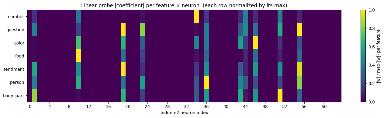
Figure 4: Heat map of linear-probe coefficients across the alive neurons (rows are features, each normalized by its max). Overlapping patterns indicate polysemantic neurons and distributed codes. For example, sentiment is read from at least 5 neurons (1, 19, 36, 46, 55), and neuron 19 carries weight for four features (question, food, sentiment, body_part).
This raises the question: what if we explicitly enforce superposition by shrinking the layer?
I varied the layer width \(k\) in \([2, 16]\) and, for each feature, classified the outcome (with threshold \(\tau = 0.85\)):
- both — linear probe accuracy \(\ge \tau\) and head accuracy \(\ge \tau\): already linearly separable at this layer.
- head only — head \(\ge \tau\) but probe \(< \tau\): non-linearly encoded at the layer, yet separable by the end of the network. This is the regime the puzzle is about.
- neither — both \(< \tau\): the feature is not learned at this \(k\).
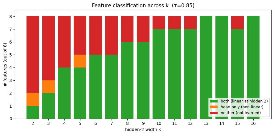
Figure 5: Per-feature outcome across \(k\). As \(k\) shrinks, “head only” and “neither” grow at the expense of “both” — capacity pressure drives non-linear encoding.
The width \(k\) imposes a bottleneck on the whole model, not just the studied layer:
- When \(k\) is large enough (\(k \ge 13\)), both the head and the layer learn cleanly separable representations across features (the long green bar).
- As \(k\) shrinks, more features become inseparable (the growing red bar).
The most interesting case is the occasional head only outcome: the layer fails to represent a feature linearly, yet the head still classifies it correctly — exactly what we saw with country in Q1 and Q2. For instance, at \(k=5\), question is linearly separable in the 2D embedding but food is not, even though the head gets both right.
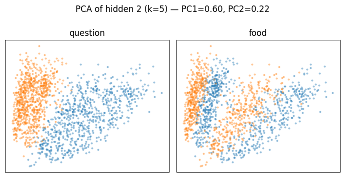
Figure 6: 2D embeddings at \(k=5\). question (left) is linearly separable; food (right) is not, yet the head still classifies it correctly.
Idea 2: Concentric shells via auxiliary losses
Next, instead of squeezing capacity, we directly shape the hidden geometry through the loss. The target: push the two classes onto concentric shells — nested spheres sharing a centroid but sitting at different radii.
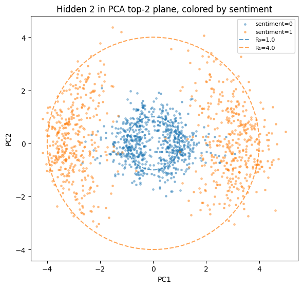
Figure 7: The concentric-shells geometry. Class 0 (blue) collapses to an inner shell at radius \(R_0 = 1\); class 1 (orange) spreads onto an outer shell at \(R_1 = 4\). The classes are linearly inseparable but quadratically separable.
Three ingredients produce this structure:
- The two class centroids should be close to each other (so the shells are concentric).
- Points of different classes should sit at different distances from that shared centroid.
- Points of the same class should be equidistant from the centroid.
We encode this with two auxiliary loss terms. Let \(R_0\) and \(R_1\) be the target radii for the two classes, and let \(\mu_0, \mu_1\) be the class centroids (mean activation per class).
Centroid-gap loss captures ingredient 1 — it pulls the two centroids together:
\[\mathcal{L}_{\text{centroid}} = \lVert \mu_1 - \mu_0 \rVert^2\]Radial loss captures ingredients 2 and 3 — it drives each point to its class’s target radius. With \(h^{(c)}i\) the batch-centered activation of sample \(i\) and \(R{y_i}\) its target radius:
\[\mathcal{L}_{\text{radial}} = \frac{1}{N}\sum_{i=1}^{N} \big( \lVert h^{(c)}_i \rVert - R_{y_i} \big)^2\]In words, \(\mathcal{L}{\text{radial}}\) pulls class-1 points to radius \(R_1\) and class-0 points to \(R_0\). The total loss is a weighted sum with the task loss \(\mathcal{L}{\text{main}}\) (binary cross-entropy):
\[\mathcal{L} = \mathcal{L}_{\text{main}} + \alpha\, \mathcal{L}_{\text{radial}} + \beta\, \mathcal{L}_{\text{centroid}}\]Injecting linear inseparability. Applying this to sentiment (chosen for illustration) with \(\alpha = 0.1\), \(\beta = 0.05\), we open a large gap: the linear probe scores 0.59 on sentiment while the model’s own head scores 0.98.
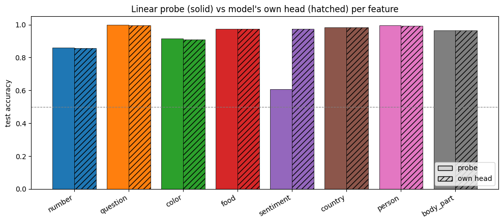
Figure 8: Test accuracy of the linear probe vs. the model’s own head, per feature (\(\alpha = 0.1\), \(\beta = 0.05\)). Only the targeted feature sentiment shows a large probe-vs-head gap; the rest are untouched.
Ablation. Both loss terms are necessary.
Removing \(\mathcal{L}_{\text{radial}}\) (set \(\alpha = 0\)) collapses the gap — probe and head both score ~0.98. Without a radial pull, points are no longer pushed to different distances, and the two classes scatter and re-mix.
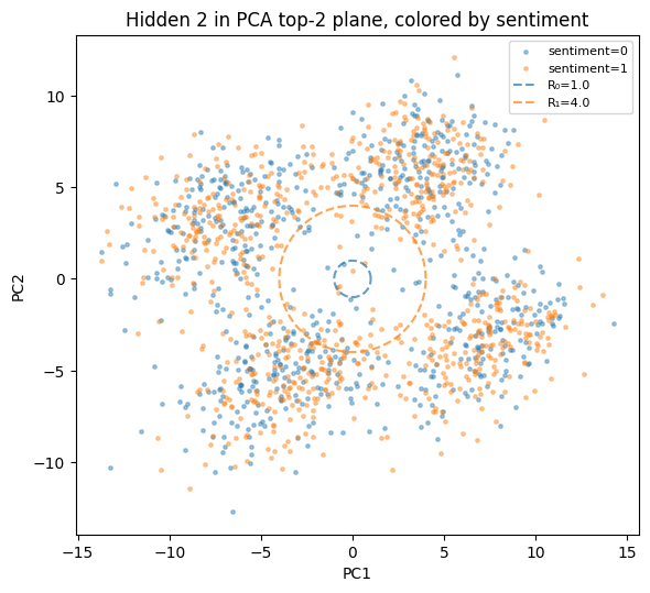
Figure 9: PCA after ablating \(\mathcal{L}_{\text{radial}}\) (\(\alpha = 0\)). Without the radial pull the two classes mix.
Removing \(\mathcal{L}_{\text{centroid}}\) (set \(\beta = 0\)) also collapses the gap — both models reach ~1.0. Curiously, in the 2D PCA plane the shells still look perfectly concentric. But in the full 64-D space they are not: the inner and outer clouds are also offset along a hidden direction that the 2D projection collapses, so a linear probe recovers them easily.
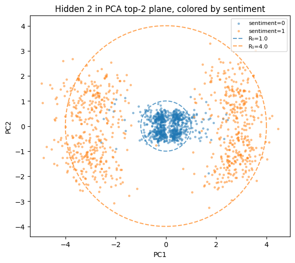
Figure 10: PCA after ablating \(\mathcal{L}_{\text{centroid}}\) (\(\beta = 0\)). The rings look concentric in 2D, but the classes stay linearly separable along a hidden direction the projection hides.
Idea 3: Gradient reversal (a failed attempt)
The last idea failed, but the lessons are worth sharing.
Both approaches above prescribe a specific geometry. Gradient reversal instead says only “do not form a linearly separable representation,” leaving the geometry open — potentially more general. The idea is borrowed from adversarial ML:
- A proxy linear probe is trained inside the loop to decode the target feature from the hidden representation.
- But before the probe’s gradient reaches the encoder, we flip its sign, so the encoder is pushed to make the probe’s job harder.
Concretely, with hidden representation \(h\), full 8-feature labels \(y_{\text{all}}\), and the target feature’s label \(y_F\):
\[\mathcal{L}_{\text{main}} = \text{BCE}\big(\text{head}(h),\ y_{\text{all}}\big) \qquad \mathcal{L}_{\text{probe}} = \text{BCE}\big(\text{probe}(h),\ y_F\big)\]The probe minimizes \(\mathcal{L}_{\text{probe}}\). The encoder and head minimize a combined loss in which the probe’s gradient is sign-flipped by a gradient-reversal layer (GRL) — identity on the forward pass, sign-flip on the backward pass:
\[\mathcal{L} = \mathcal{L}_{\text{main}} + \lambda \cdot \text{GRL}\big(\mathcal{L}_{\text{probe}}\big)\]where \(\lambda\) controls the adversarial pressure. We expected linearly inseparable representations, and hence worse linear probes than the head. It did not work out. Two observations:
Observation 1. The in-loop probe’s accuracy hovers near 0.5 (chance), but a fresh held-out probe trained on the same representations recovers the feature at ~0.9 — and this gap persists throughout training. The encoder is dodging the specific in-loop probe rather than genuinely scrubbing the feature.
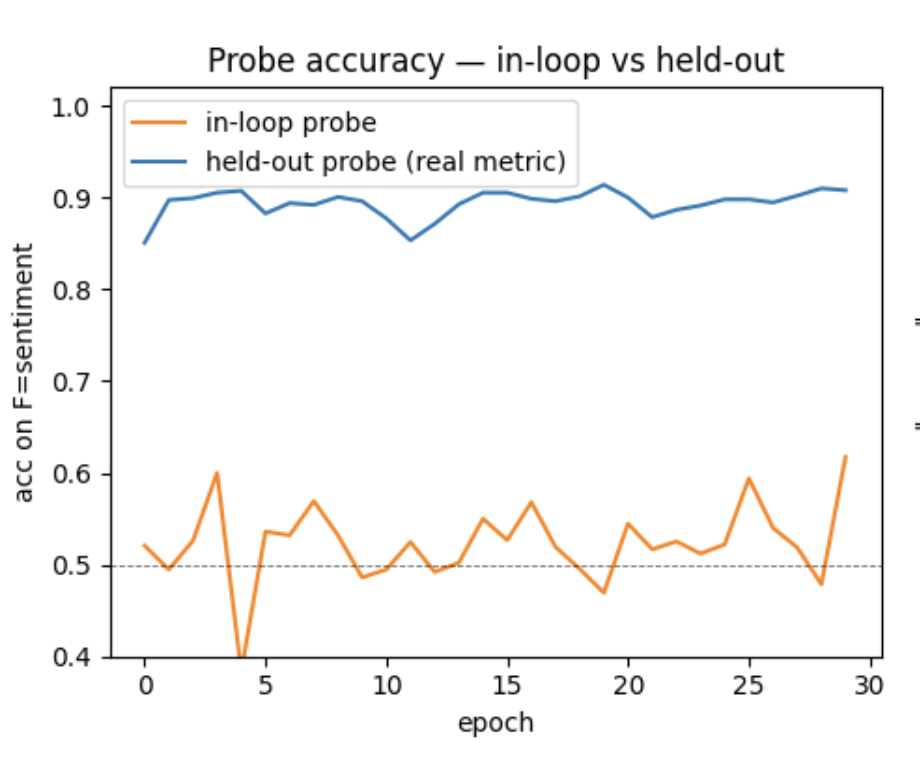
Figure 11: In-loop probe accuracy stays near chance while a held-out probe recovers sentiment throughout training — evidence the encoder dodges the particular probe rather than removing the feature.
Observation 2. The head ends up worse than the held-out linear probe on the target feature — the opposite of the intended gap. This was the biggest surprise.
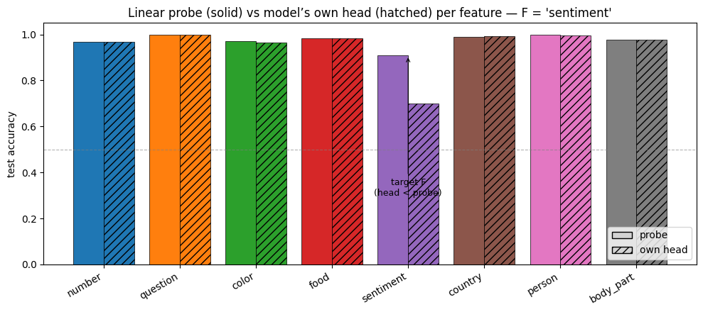
Figure 12: Per-feature test accuracy after GRL training on sentiment. On the target feature the head (hatched) is worse than a held-out linear probe (solid) — the reverse of what we wanted.
Takeaways
Linear separability is just one way a network can lay out a feature. This puzzle made that concrete from three directions:
- Capacity alone can force non-linear encoding — squeeze the layer and features start sharing neurons in superposition.
- Loss geometry can sculpt a feature onto a prescribed surface (concentric shells), producing a clean probe-vs-head gap — but every ingredient has to pull its weight, as the ablations show.
- Adversarial pressure against a single in-loop probe is brittle: the encoder learns to dodge that probe rather than remove the feature, a cautionary tale for probing-based safety methods.
For interpretability, the practical reminder is that a failed linear probe does not mean a feature is absent — it may just be encoded on a surface your probe can’t see.
Full details, extra plots, and code are in the original write-up and at xiaohan2012/bluedot-tais-puzzle.
